Generated using ptrv/gpx2spatialite, rendered in QGIS as lines with 75% transparency.
Generated using ptrv/gpx2spatialite, rendered in QGIS as lines with 75% transparency.
 @MaptimeTO asked me to summarize the brief talk I gave last week at Maptime Toronto on making maps from the Technical and Administrative Frequency List (TAFL) radio database. It was mostly taken from posts on this blog, but here goes:

I’ve used Shapely before for more sensible things, but it’s a dab hand at driving anything Cartesian — like my old HP-7470A pen plotter. Here’s some crude code to draw shapes and hatches in HP-GL: hpgl-shapely_hatch.py.
More silliness like this in my other blog under the plotter tag.

André shows you how to add the OSGB New Popular Edition maps of England as a TMS layer in QGIS.
Today, I’m going to describe how I get fairly accurate buffer distances over a really large area.
But first, I’m going to send a huge look of disapproval (![]() ) to Norway. It’s not for getting all of the oil and finding a really mature way of dealing with it, and it’s not for the anti-personnel foods (rancid fish in a can, salt liquorice, sticky brown cheese …) either. It’s for this:
) to Norway. It’s not for getting all of the oil and finding a really mature way of dealing with it, and it’s not for the anti-personnel foods (rancid fish in a can, salt liquorice, sticky brown cheese …) either. It’s for this:
The rest of the world is perfectly fine with having their countries split across Universal Transverse Mercator zones, but not Norway. “Och, my wee fjords…” they whined, and we gave them a whole special wiggle in their UTM zone. Had it not been for Norway’s preciousness, GIS folks the work over could’ve just worked out their UTM zone from a simple calculation, as every other zone is just 6° of longitude wide.
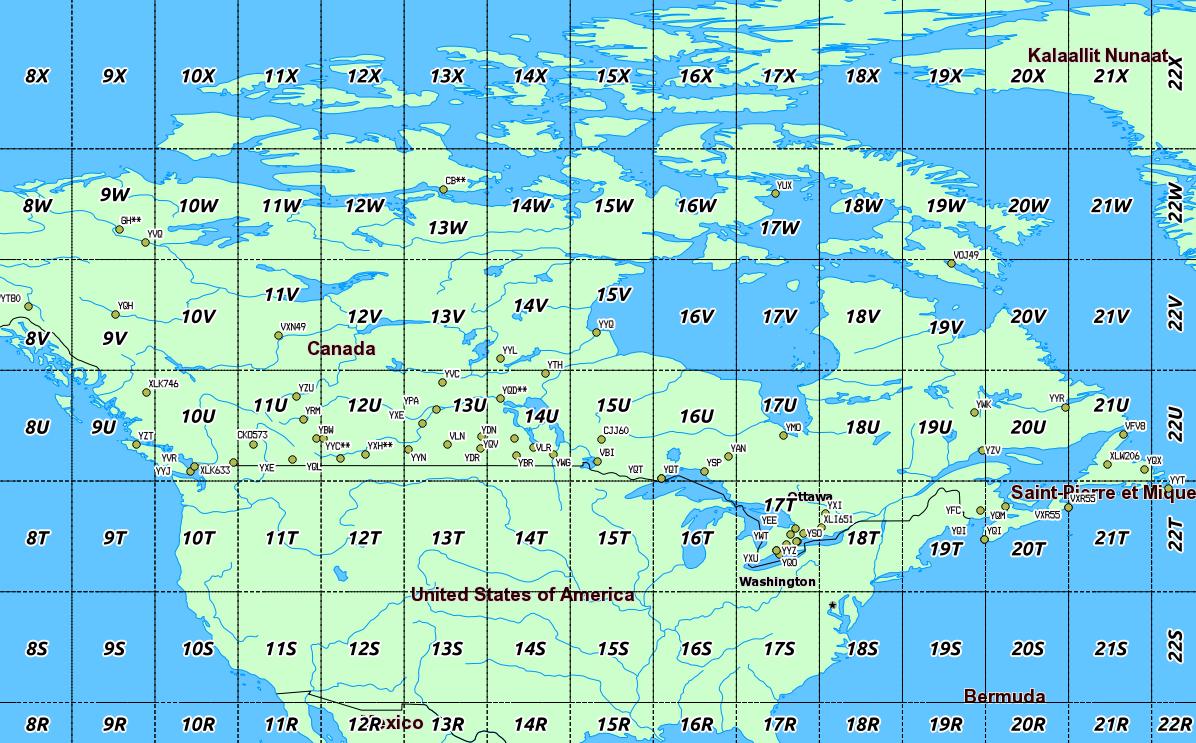
Canada has no such qualms. In a big country (dreams stay with you …), we have a lot of UTM zones:
 We’re in zones 8–22, which is great if you’re working in geographic coordinates. If you’re unlucky enough to have to apply distance buffers over a long distance, the Earth is inconveniently un-flat, and accuracy falls apart.
What we can do, though, is transform a geographic coordinate into a projected one, apply a buffer distance, then transform back to geographic again. UTM zones are quite good for this, and if it weren’t for bloody Norway, it would be a trivial process. So first, we need a source of UTM grid data.
Well, the Global UTM Zones Grid from EPDI looks right, and it’s CC BY-NC-SA licensed. But it’s a bit busy with all the grid squares:
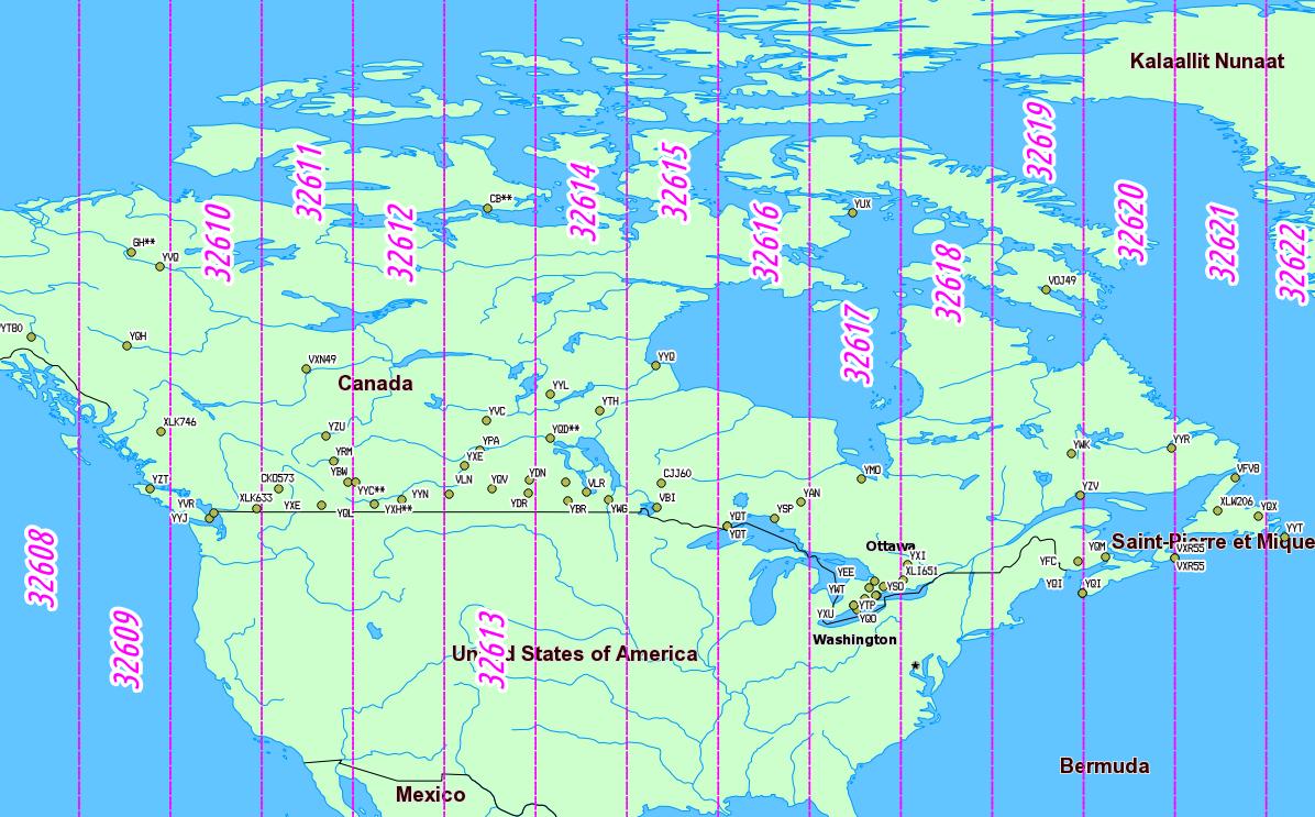
 What’s more, there’s no explicit way of getting the numeric zone out of the CODE field (used as labels above). We need to munge this a bit. In a piece of gross data-mangling, I’m using an awk (think: full beard and pork chops) script to process a GeoJSON (all ironic facial hair and artisanal charcuterie) dump of the shape file. I’m not content to just return the zone number; I’m turning it into the EPSG WGS84 SRID of the zone, a 5-digit number understood by proj.4:
32hzz
where:
I live in Zone 17 North, so my SRID is 32617.
Here’s the code to do it: zones_add_epsg-awk (which you’ll likely have to rename/fix permissions on). To use it:
And, lo!
 So we can now load this wgs84utm shapefile as a table in SpatiaLite. If you wanted to find the zone for the CN Tower (hint: it’s the same as me), you could run:
select EPSGSRID from wgs84utm where within(GeomFromText('POINT(-79.3869585 43.6425361)',4326), geom);
which returns ‘32617’, as expected.
(I have to admit, I was amazed when this next bit worked.)
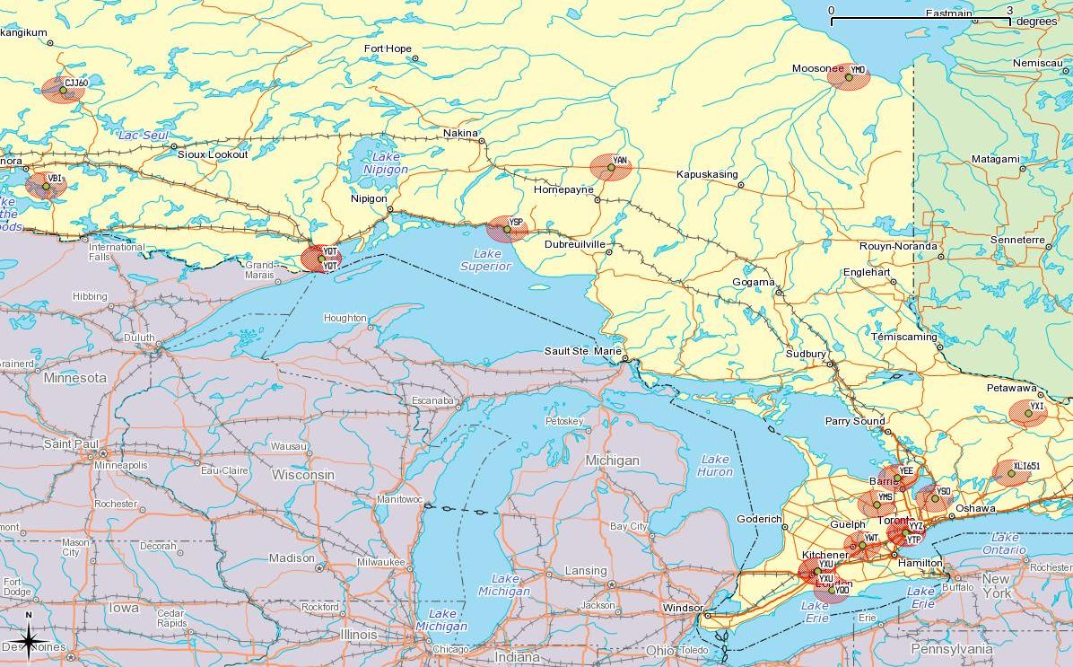
Let’s say we have to identify all the VOR stations in Canada, and draw a 25 km exclusion buffer around them (hey, someone might want to …). VOR stations can be queried from TAFL using the following criteria:
This can be coded as:
SELECT * FROM tafl WHERE licensee LIKE 'NAV CANADA%' AND tx >= 108 AND tx <= 117.96 AND location LIKE '%VOR%';which returns a list of 67 stations, from VYT80 on Mount Macintyre, YT to YYT St Johns, NL. We can use this, along with the UTM zone query above, to make beautiful, beautiful circles:
SELECT tafl.PK_ROWID, tafl.tx, tafl.location, tafl.callsign, Transform (Buffer ( Transform ( tafl.geom, wgs84utm.epsgsrid ), 25000 ) , 4326 ) AS bgeom FROM tafl, wgs84utm WHERE tafl.licensee LIKE 'NAV CANADA%' AND tafl.tx >= 108 AND tafl.tx < 117.96 AND tafl.location LIKE '%VOR%' AND Within( tafl.geom, wgs84utm.geom );Ta-da!
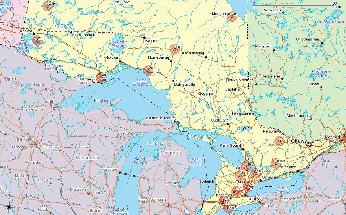
Yes, they look oval; don’t forget that geographic coordinates don’t maintain rectilinearity. Transformed to UTM, they look much more circular:
Update, 2017: TAFL now seems to be completely dead, and Spectrum Management System has replaced it. None of the records appear to be open data, and the search environment seems — if this is actually possible — slower and less feature-filled than in 2013.
Update, 2013-08-13: Looks like most of the summary pages for these data sets have been pulled from data.gc.ca; they’re 404ing. The data, current at the beginning of this month, can still be found at these URLs:
I build wind farms. You knew that, right? One of the things you have to take into account in planning a wind farm is existing radio infrastructure: cell towers, microwave links, the (now-increasingly-rare) terrestrial television reception.
I’ve previously written on how to make the oddly blobby shape files to avoid microwave links. But finding the locations of radio transmitters in Canada is tricky, despite there being two ways of doing it:
So searching for links is far from obvious, and it’s not like wireless operators do anything conventional like register their links on the title of the properties they cross … so these databases are it, and we must work with them.
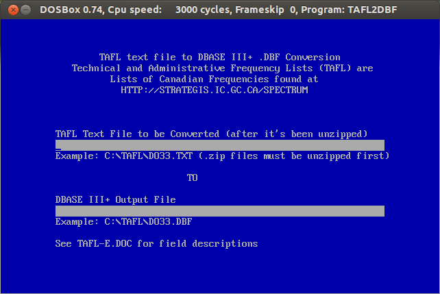
The good things is that TAFL is now Open Data, defined by a reasonable Open Government Licence, and available on the data.gc.ca website. Unfortunately, the official Industry Canada tool to process and query these files, is a little, uh, behind the times:Yes, it’s an MS-DOS exe. It spits out DBase III Files. It won’t run on Windows 7 or 8. It will run on DOSBox, but it’s rather slow, and fails on bigger files.
That’s why I wrote taflmunge. It currently does one thing properly, and another kinda-sorta:
taflmunge runs anywhere SpatiaLite does. I’ve tested it on Linux and Windows 7. It’s just a SQL script, so no additional glue language required. The database can be queried on anything that supports SQLite, but for real spatial cleverness, needs SpatiaLite loaded. Full instructions are in the taflmunge / README.md.
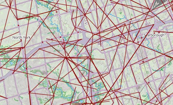
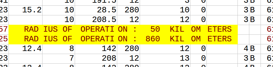
TAFL is clearly maintained by licensees, as the data can be a bit “vernacular”. Take, for example, a tower near me:
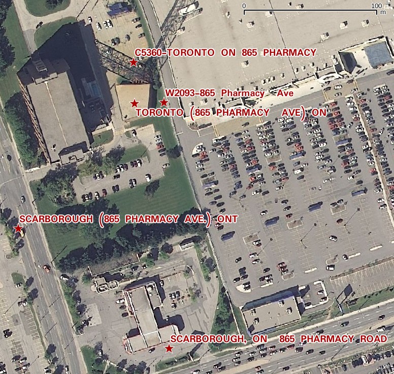
The tower is near the top of the image, but the database entries are spread out by several hundred meters. It’s the best we’ve got to work with.
Ultimately, I’d like to keep this maintained (the Open Data TAFL files are updated monthly), and host it in a nice WebGIS that would allow querying by location, frequency, call sign, operator, … But that’s for later. For now, I’ll stick with refining it locally, and I hope that someone will find it useful.
Visualizing where the data flows without wires. Extracted from the Ontario Technical and Administrative Frequency List (TAFL), and used under the Open Government Licence – Canada.
It was Doors Open Toronto last weekend, and the city published the locations as open data: Doors Open Toronto 2013. I thought I’d try to geocode it after Richard suggested we take a look. OpenStreetMap has the Nominatim geocoder, which you can use freely as long as you accept restrictions on bulk queries.
As a good and lazy programmer, I first tried to find pre-built modules. Mistake #1; they weren’t up to snuff:
So I rolled my own, using nowt but the Nominatim Search Service Developer’s Guide, and good old simple modules like URI::Escape, LWP::Simple, and JSON::XS. Much to my surprise, it worked!
Much as I love XML, it’s a bit hard to read as a human, so I smashed the Doors Open data down to simple pipe-separated text: dot.txt. Here’s my code, ever so slightly specialized for searching in Toronto:
#!/usr/bin/perl -w
# geonom.pl - geocode pipe-separated addresses with nominatim
# created by scruss on 02013/05/28

use strict;
use URI::Escape;
use LWP::Simple;
use JSON::XS;

# the URL for OpenMapQuest's Nominatim service
use constant BASEURI => 'http://open.mapquestapi.com/nominatim/v1/search.php';

# read pipe-separated values from stdin
# two fields: Site Name, Street Address
while (<>) {
    chomp;
    my ( $name, $address ) = split( '\|', $_, 2 );
    my %query_hash = (
        format  => 'json',
        street  => cleanaddress($address),    # decruft address a bit
                                              # You'll want to change these ...
        city    => 'Toronto',                 # fixme
        state   => 'ON',                      # fixme
        country => 'Canada',                  # fixme
        addressdetails => 0,                  # just basic results
        limit          => 1,                  # only want first result
             # it's considered polite to put your e-mail address in to the query
             # just so the server admins can get in touch with you
        email => 'me@mydomain.com',    # fixme

        # limit the results to a box (quite a bit) bigger than Toronto
        bounded => 1,
        viewbox => '-81.0,45.0,-77.0,41.0'    # left,top,right,bottom - fixme
    );

    # get the result from Nominatim, and decode it to a hashref
    my $json = get( join( '?', BASEURI, escape_hash(%query_hash) ) );
    my $result = decode_json($json);
    if ( scalar(@$result) > 0 ) {             # if there is a result
        print join(
            '|',    # print result as pipe separated values
            $name, $address,
            $result->[0]->{lat},
            $result->[0]->{lon},
            $result->[0]->{display_name}
          ),
          "\n";
    }
    else {          # no result; just echo input
        print join( '|', $name, $address ), "\n";
    }
}
exit;

sub escape_hash {

    # turn a hash into escaped string key1=val1&key2=val2...
    my %hash = @_;
    my @pairs;
    for my $key ( keys %hash ) {
        push @pairs, join( "=", map { uri_escape($_) } $key, $hash{$key} );
    }
    return join( "&", @pairs );
}

sub cleanaddress {

    # try to clean up street addresses a bit
    # doesn't understand proper 'Unit-Number' Canadian addresses tho.
    my $_ = shift;
    s/Unit.*//;     # shouldn't affect result
    s/Floor.*//;    # won't affect result
    s/\s+/ /g;      # remove extraneous whitespace
    s/ $//;
    s/^ //;
    return $_;
}
It quickly became apparent that the addresses had been entered by hand, and weren’t going to geocode neatly. Here are some examples of the bad ones:
Curiously, some (like the address for Black Creek Pioneer Village) were right, but just not found. Since the source was open data, I put the right address into OpenStreetMap, so for next year, typos aside, we should be able to find more events.
Now, how accurate were the results? Well, you decide:
ClickFu is dead in QGIS 3. Please try to forget how useful it was. nextgis / clickfu appears to be an updated version, but it has old QT dependencies and no longer works either.
Since QGIS 1.8 took the rather boneheaded move of hiding all the plugin sources except the official one, here’s how to get the other repositories back:
Now you can add all the plugins!
ClickFu is kind of magic. It allows you to choose an online map service, click anywhere on your GIS viewport, and the correct location link opens in your browser. Very handy for sharing locations with people who don’t have a GIS setup. It properly takes coordinate reference systems into account, too, so no messing about with datum shifts and the like.
Another plugin that hasn’t made it to the official repo is Luiz Motta’s Zip Layers. It still lurks at http://pyqgis.org/repo/contributed.
Click Fu runs just fun under QGIS 2.2 – as long as you remember to delete any pre-2.0 versions and then reinstall.