Categories
Uncategorized

too damn many open data licences

Oh Canada …

  1. Open Government Licence – Ontario
  2. City of Guelph Open Government Licence
  3. Open Government Licence – Vancouver
  4. Open Government Licence – County of Grande Prairie
  5. Open Government Licence – Alberta
  6. Open Government Licence for City of Nanaimo
  7. Open Government Licence – Strathcona County
  8. Open Data Licence for Town of Banff
  9. Open Government Licence for District of Squamish
  10. Open Government Licence — Town of Oakville
  11. Open Government Licence – Kamloops
  12. Open Government License for the City of Surrey
  13. Open Government Licence – Toronto
  14. OPEN GOVERNMENT LICENCE – TORONTO PUBLIC LIBRARYand yes, they’re not covered by the City’s licence
  15. Open Government License for Government of British Columbia
  16. City of Edmonton Open Data Terms of Usea truly odd one that seems to have little in common with any of the others
  17. Region of Waterloo – Open Data Licence
  18. Open Government Licence for the City of Regina
  19. Open Government Licence – The Corporation of the City of Kitchener
  20. York Region’s Open Data Licencea catchy little URL at only 427 characters short
  21. Open Data Licence for The Regional Municipality of Peel
  22. Open Government Licence – Canada
  23. Open Government Licence – City of Ottawa

— and they’re all slightly different, even in how they spell the word “Licence”  …

Categories
Uncategorized

Summary of my off-the-cuff Maptime Presentation: Canadian Microwave Links

Screenshot from 2014-07-26 10:17:15@MaptimeTO asked me to summarize the brief talk I gave last week at Maptime Toronto on making maps from the Technical and Administrative Frequency List (TAFL) radio database. It was mostly taken from posts on this blog, but here goes:

  1. One of the many constraints in building wind farms is allowing for radio links. Both the radio and the wind industries have agreed on a process of buffering and consultation. Here’s how I handled it in Python: Making weird composite shapes with Shapely.
  2. The TAFL databases — which contains locations and technical data for all licensed transmitters — are now open data. You can find them here: Technical and Administrative Frequency List (TAFL).
  3. The format is a real delight for all legacy-data nerds: aka a horrible mess of conditional field widths and arcane numeric codes. I wrote a SpatiaLite SQL script to make sense of it all: scruss/taflmunge. This (kind of) explains what it does: TAFL — as a proper geodatabase.
  4. Here’s a raw dump (very little metadata, sorry) from 2013 in the wonderful uMap: Ontario Microwave Links.
  5. In a fabulous piece of #opendatafail, Industry Canada have migrated all the microwave data (so, all links ≥ 960 MHz) to a new system which doesn’t work yet, and also stripped out all of the microwave data from recent TAFL files. They claim to be fixing it, but don’t hold your breath. If you want data to play with, here’s Ontario’s data from October 2013 (nb: huge) — ltaf_ont_tafl-20131001.
Categories
GIS Uncategorized

TAFL — as a proper geodatabase

Update, 2017: TAFL now seems to be completely dead, and Spectrum Management System has replaced it. None of the records appear to be open data, and the search environment seems — if this is actually possible — slower and less feature-filled than in 2013.

Update, 2013-08-13: Looks like most of the summary pages for these data sets have been pulled from data.gc.ca; they’re 404ing. The data, current at the beginning of this month, can still be found at these URLs:

I build wind farms. You knew that, right? One of the things you have to take into account in planning a wind farm is existing radio infrastructure: cell towers, microwave links, the (now-increasingly-rare) terrestrial television reception.

I’ve previously written on how to make the oddly blobby shape files to avoid microwave links.  But finding the locations of radio transmitters in Canada is tricky, despite there being two ways of doing it:

  1. Wrestle with the Spectrum Direct website, which can’t handle the large search radii needed for comprehensive wind farm design. At best, it spits out weird fixed-width text data, which takes some effort to parse.
  2. Download the Technical and Administrative Frequency Lists (TAFL; see update above for URLs), and try to parse those (layout, fields). Unless you’re really patient, or have mad OpenRefine skillz, this is going to be unrewarding, as the files occasionally drop format bombs like
    never do this, okay?
    Yes, you just saw conditional different fixed-width fields in a fixed-width text file. In my best Malcolm Tucker (caution, swearies) voice I exhort you to never do this.

So searching for links is far from obvious, and it’s not like wireless operators do anything conventional like register their links on the title of the properties they cross … so these databases are it, and we must work with them.

The good things is that TAFL is now Open Data, defined by a reasonable Open Government Licence, and available on the data.gc.ca website. Unfortunately, the official Industry Canada tool to process and query these files, is a little, uh, behind the times:tafl2dbfYes, it’s an MS-DOS exe. It spits out DBase III Files. It won’t run on Windows 7 or 8. It will run on DOSBox, but it’s rather slow, and fails on bigger files.

That’s why I wrote taflmunge. It currently does one thing properly, and another kinda-sorta:

  1. For all TAFL records fed to it, generates a SpatiaLite database containing these points and all their data; certainly all the fields that the old EXE produced. This process seems to work for all the data I’ve fed to it.
  2. Tries to calculate point-to-point links for microwave communications. This it does less well, but I can see where the SQL is going wrong, and will fix it soon.

taflmunge runs anywhere SpatiaLite does. I’ve tested it on Linux and Windows 7. It’s just a SQL script, so no additional glue language required. The database can be queried on anything that supports SQLite, but for real spatial cleverness, needs SpatiaLite loaded. Full instructions are in the taflmunge / README.md.

TAFL is clearly maintained by licensees, as the data can be a bit “vernacular”. Take, for example, a tower near me:

pharm_eg

The tower is near the top of the image, but the database entries are spread out by several hundred meters. It’s the best we’ve got to work with.

Ultimately, I’d like to keep this maintained (the Open Data TAFL files are updated monthly), and host it in a nice WebGIS that would allow querying by location, frequency, call sign, operator, … But that’s for later. For now, I’ll stick with refining it locally, and I hope that someone will find it useful.

Categories
GIS

Styling GeoBase land cover data

GeoBase provides the free Land Cover, Circa 2000 – Vector product which contains 1:250,000 land cover categories (water, ice, crops, urban, trees, …) for all of Canada. It has some use in wind energy development, as you can use it to classify the roughness length of terrain for flow modelling.

The data are provided as very large shape files, indexed by National Topographic System (NTS) codes. These aren’t the easiest to remember, so I keep finding myself going back to the Vector Indexes of the National Topographic System of Canada, especially the handy Google Earth version. Toronto is in NTS 030M, so I downloaded that. Here is what a cropped part looks like loaded over the local Toporama WMS tiles:

The fun stuff is hidden in the attribute table:

So the COVTYPE field is clearly holding something about the land cover type. But what?

GeoBase helpfully provide a PDF key and a style file — which only works with ArcGIS products. As a dedicated (okay, yes, cheap) user of Open GIS systems, this could not stand! So I dug through the Styled Layer Descriptor (SLD) format, and came up with style files (in both English & French) that work with QGIS: SLD_LCC2000-V-en_CSC2000-V-fr.zip.

To use them with QGIS, open up the layer properties, and go to the Style tab. You want to use the New Symbology option, then Load Style … From here, you can open the SLD file (changing the file type from QGIS’s default QML to SLD), which should appear like this:

This makes the layer look much better:

Categories
Uncategorized

The Invisible City

Now you see it …

There’s not a whole lot north of North Bay. Highway 11 winds through some extensive geometry, but few habitations. Until something wonderful (and quite a bit wrong) happened at 46° 31′ 21″ N, 79° 33′ 9″ W on OpenStreetMap. A whole new town about 25 minutes out of North Bay sprung up overnight — and was as quickly deleted as mappers caught and reverted the vandalism.

Now you don’t.

The misguided mapper put quite a lot of work into this ephemeral town. It’s got urban rail, parklands, residential areas and more. You can see the detail on this large image of the town (650 KB PNG). If you want to play with the data, here’s a zipped OSM XML file of the area before it was reverted. But please, don’t re-upload it; OpenStreetMap should be for real features on the ground, and not for confusing map data consumers.

Thanks to Bootprint for noticing this, and to rw__ for reverting the edits.

Categories
GIS

Awesome USGS orthoimagery … in Canada?

Update, 2015: I don’t think this coverage works any more. The WMS data was carefully trimmed to the US border last time I looked.

Detail of Erie Shores Wind Farm showing USGS orthophotos from WMS

I was trying to do some OpenStreetMap edits in rural southern Ontario, but the default Bing background aerial imagery is very poor. Clicking around in semi-plokta mode to find better images, I happened upon “OSM US USGS Large Scale Aerial Imagery”, which loaded up some beautiful and recent pictures. I guess that since we’re close to the border, the USGS doesn’t bother to trim its images too close.

Ian Dees, who admins the particular OSM server, confirmed that these are from The National Map‘s TNM_Large_Scale_Imagery service; thanks, Ian! These images are at least as good for my purposes as the SWOOP data — except not $50/km2, and without elaborate usage restrictions.

Categories
GIS

geocoder.ca’s excellent database

Update, late 2017: Looks like geocoder.ca’s database hasn’t been updated since late 2015. The download link is still active, though.

geocoder.ca provides a crowdsourced postal code geocoder under the ODbL. You can download the database as CSV directly. Here’s a bash script to convert that text file into a (very large) point shapefile:

#!/bin/bash
# geocoder2shp.sh - convert geocoder.ca CSV to a shape file
# NB: input CSV is UTF-8; it is passed through unchanged
# Needs >= v1.7 of GDAL
# scruss - 2012/04/15

if [ ! -f Canada.csv.gz ]
then
    echo ""
    echo " " Download \"Canada.csv.gz\" into the current directory from
    echo "  " http://geocoder.ca/onetimedownload/Canada.csv.gz
    echo " " and try again.
    echo ""
    exit 1
fi

# make input file with header
echo PostalCode,Latitude,Longitude,City,Province > Canada2.csv
gunzip -c Canada.csv.gz >> Canada2.csv

# create GDAL VRT file
cat > Canada2.vrt <<EOF
<OGRVRTDataSource>
  <!-- note that OGRVRTLayer name must be basename of source file -->
  <OGRVRTLayer name="Canada2">
    <SrcDataSource>Canada2.csv</SrcDataSource>
    <GeometryType>wkbPoint</GeometryType>
    <LayerSRS>EPSG:4326</LayerSRS>
    <GeometryField encoding="PointFromColumns" x="Longitude" y="Latitude"/>
    <Field name="PostalCode" type="String" width="6" />
    <Field name="Latitude" type="Real" />
    <Field name="Longitude" type="Real" />
    <Field name="City" type="String" width="60" />
    <Field name="Province" type="String" width="2" />
  </OGRVRTLayer>
</OGRVRTDataSource>
EOF

# create shapefile
ogr2ogr PostalCodes.shp Canada2.vrt

# clean up
rm -f Canada2.csv	Canada2.vrt

Though the script is a bit Unix-centric, it’s just a simple list of instructions which could be run on any command line. What it does is add some headers to the geocoder.ca file, then sets up an OGR Virtual Format to convert the text into a fairly well-defined shapefile. When you use this shapefile, you should credit geocoder.ca as the ODbL requires.

Eek! geocoder.ca has been sued by Canada Post! (News responses: Michael Geist, Boing Boing, CBC) I’ve donated to defend this useful service.

Categories
GIS

we can has street names

Pierre Béland reminded the Canadian OSM group of the GeoBase WMS, which has all the NRN road names in it. Here’s my neighbourhood’s OpenStreetMap data with the road names overlaid.

Categories
GIS

image georeferencing with QGIS

Quantum GIS (QGIS) has a very powerful image georeferencing module. What that allows you to do is convert screen pixels to a map of an area. The pixels could be from a scanned map or from a screen image. Scanned maps can sometimes be a little distorted, but QGIS’s georeferencer can handle that, within limits.

For an example, say I live in Redickville, ON (I don’t, but some folks do). I’ve heard from North Dufferin Agricultural & Community Taskforce (NDACT) that a large quarry is planned in my area. How close am I going to be from it?

NDACT has a helpful map (2.4 MB PNG image) had a helpful map (which I’ve kept here so you can work through this: MelancthonAerial), but it has no scale. It’s clearly derived from something like Google Maps, so it’s not exactly a free image I can throw about. One thing about georeferencing is that both the source image and the map from which you take you control points affect the licensing of the final map. You’re ending up with a derived work.

There are lots of sources of coordinates for your control points. You could always use Google Maps, but then you’re well down the derived work sinkhole. GeoGratis has a bunch of good data sources, and they are free to use. I’m going to use Toporama‘s digital image maps, as they’re clear and fairly accurate.

Redickville is on Toporama sheet 041A01. I’ve downloaded it as UTM, as it’s easier to measure distances that way. You want to set up your project so it uses the coordinate reference system (CRS) that the control point map uses. Toporama uses EPSG 26917 in the area (easily checked with gdalinfo; it’ll come up with something like AUTHORITY[“EPSG”,”26917″]]), so you should set the project to use that CRS:

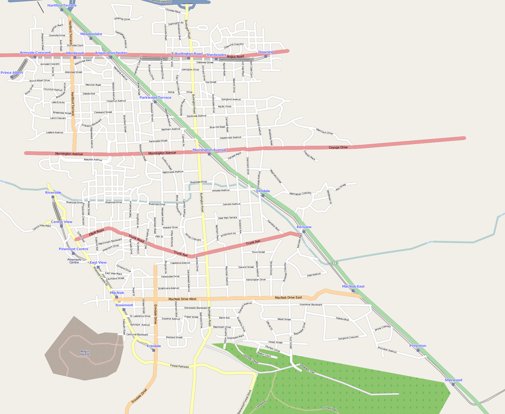
And here’s the raster map loaded into QGIS;

Opening up the georeferencer plugin (which is now in the Raster menu, as of QGIS 1.8) gives you a whole lot of blank:

If we open the raster, you can zoom into the area into which you want to put control points. You want to have the highest zoom that the map’s still clear, as the accuracy of your final map depends on how well you placed control points. I’ve chosen road intersections as my control points. Here are the ones I’m going to use:

Point   E-W Road        N-S Road        Note
1       County Rd 21    2nd Line W      Honeywood
2       County Rd 21    4th Line       
3       20th Side Rd    5th Line       
4       15th Side Rd    County Rd 124   just S of where 124 straightens
5       15th Side Rd    Mulmur Townline
6       4th Line        5th Line        4th Line really runs SE-NW

These intersections are fairly well spaced apart, and are clear on both maps. So I choose a pixel on the map in the georeferencer, and a dialogue comes up:

(If you’ve downloaded the MelancthonAerial archive from here, the georeferencing points should load automatically from the “Melancthon Aerial July 22 09.png.points” file. If you want to go through the exercise of manually adding reference points, delete the points file.)

Here I’ve already clicked on the corresponding point on the Toporama map, and the coordinates have been filled in. If you know the coordinates, you can enter them in the boxes. Once you click OK, you have your first control point:

We can add the rest one by one. QGIS’s “Zoom Previous” is really useful for flipping between scales on both the plugin window and the main map. It’s probably a good idea to “Save GCP Points As …” every now and again so you don’t lose your work. Here are all of the points in the georeferencer plugin:

Now you want to modify the Transformation Settings; it’s the little wrench/spanner in the toolbar:

There are lots of options here:

  • Transformation Type: Linear is useful if you’re just adding georeference data to an already computer generated map. Helmert is a simple shear/scale/rotate transformation. The various Polynomial types will correct more gross distortions, but need many control points and can be processor intensive. Thin Plate Spline will distort your map locally to match GCPs; this can work well if your map’s a bit “vernacular”, but if your control points are wrong, your map will end up hilariously melty.
  • Resampling Method: This controls how the output pixels are calculated. Nearest Neighbour is quick and blocky, but useful if you’re mapping an image that has sharp transitions. Cubic maintains more detail, while applying some smoothing at the cost of some detail loss and a fair bit of processing power. The other options can look nice, but eat CPU. This is worth experimenting with many options, as there’s no one solution for all maps.
  • Compression: This controls the file size of the output GeoTiff file. JPEG and Deflate can result in small files, but there’s a chance that other GIS systems can’t read the data. Note that JPEG is lossy, and will lose some detail.

Don’t forget to set the output raster file, and make sure that the target SRS matches the CRS (EPSG 26917) you chose earlier.

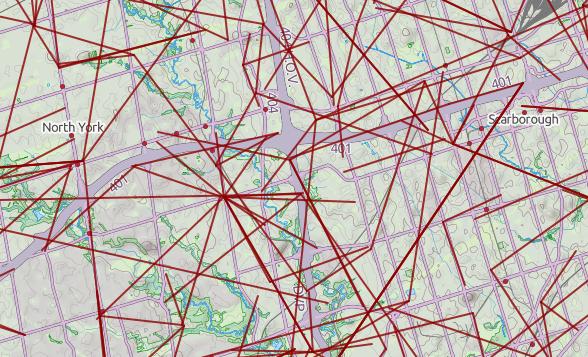
Helmert is a useful transformation type to check your work. The plugin plots the residual difference between the two sets of map control points as red lines. Here, I’ve clearly made an error in point ID 2:

If you unselect the bad point, the plugin quickly calculates the residuals again. When this one bad point is removed, the residuals drop down to less than 1.0 for each point. I’ve got enough points for a Helmert transformation with 5 GCPs, but I’d probably want some more points for more complex transformations.

Once you hit “Start Transformation”, QGIS will create your referenced image. If you’ve chosen a simple linear transformation, it won’t create a GeoTiff file, but just a world file for your image.

So here’s the georeferenced image overlaid on the Toporama map, with a bit of transparency. It’s quite a good match:

(the above’s an image saved straight from QGIS. It helpfully creates a world file too, so here it is: redickville.jpgw)

So to answer the hypothetical question, Redickville’s pretty well surrounded by this proposed quarry.

Categories
GIS

untangling CanVec

It’s almost as if NRCan doesn’t want anyone to use CanVec. I mean, it’s a free and comprehensive data set for the whole country; anyone who can type in a postal code and click a couple of times can download the CanVec map tile for where they live. But on the other hand, cracking open that download reveals an impenetrable mess of information that probably makes most users go away.

I’ve played with it before, and do occasionally drag out a layer at work, but have never got much further than that. GIS types must be very quiet, because Using CanVec – maphew and CanVec – OpenStreetMap Wiki are about the only public discussions of its content.

CanVec is delivered in two formats: Geography Markup Language (GML), and our friend, the Shapefile. While the GML version contains relatively few files, all the tools I have choke on the data. So shapefiles it is.

Opening up the archive for the Toronto area (it’s tile 030m11) I see 192 files. Four of those are (not very useful) metadata files. Realising that a shapefile ships as four files (the mandatory shp, dbf and shx files, plus the optional prj file) that’s 47 layers. The file names look a bit like this: 030m11_6_0_BS_1250009_0.shp, 030m11_6_0_BS_1370009_2.shp, 030m11_6_0_BS_2010009_0.shp. The names really do mean something:

030m11_6_0_BS_1370009_2.shp
|--+-| |+| |----+-----|
   |    |        \ Layer Code and Type
   |    \ Version
   \ Map tile

CanVec – Entity Names and Codes, Edition 1.1.0 (XLS) explains the layers, and how they relate to the shapefile names. Rather than relating unique layer codes to layer descriptions, the Entity Names & Codes document has it backwards. So I made the much simplified canvec_simple-20100523.csv which lists layer codes against attributes in a more sensible manner. I added a derived ‘name’ column, which I use for layer naming from these files. The layers use EPSG:4617 (NAD83 CSRS) coordinates.

Tip of the hat to maphew – Revision 123: /trunk/gis/canvec for providing a file that was the ‘Aha!’ moment.