Categories
GIS

GeoURIs for fun and profit

Behold the GeoURI:

geo:37.22976,-93.28663

It’s just a simple lat/long pair which some browsers (mostly mobile) will parse as locations. It probably won’t work in your desktop browser, but here’s an example as a link: Askinosie Chocolate — Springfield, MO.

You can encode case-insensitive URIs very efficiently as QR Codes. If you’re okay with ~10m resolution on your locations, you can make very tiny QR Codes indeed:

qrencode -i -o Askinosie.png 'geo:37.2298,-93.2866'

Askinosie locationI’ve half a mind to make a little GPS-enable box that prints QR Code stickers with the current location, and the caption You are here.

Categories
GIS

Styling GeoBase land cover data

GeoBase provides the free Land Cover, Circa 2000 – Vector product which contains 1:250,000 land cover categories (water, ice, crops, urban, trees, …) for all of Canada. It has some use in wind energy development, as you can use it to classify the roughness length of terrain for flow modelling.

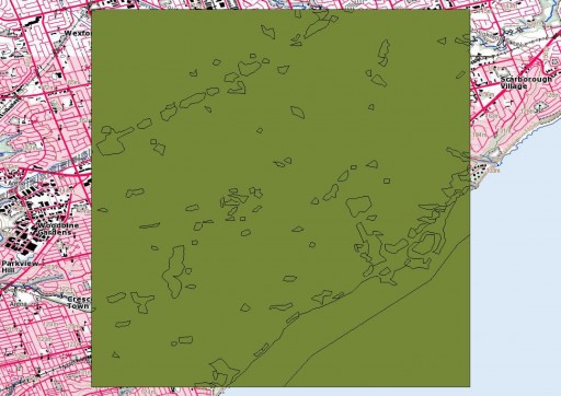
The data are provided as very large shape files, indexed by National Topographic System (NTS) codes. These aren’t the easiest to remember, so I keep finding myself going back to the Vector Indexes of the National Topographic System of Canada, especially the handy Google Earth version. Toronto is in NTS 030M, so I downloaded that. Here is what a cropped part looks like loaded over the local Toporama WMS tiles:

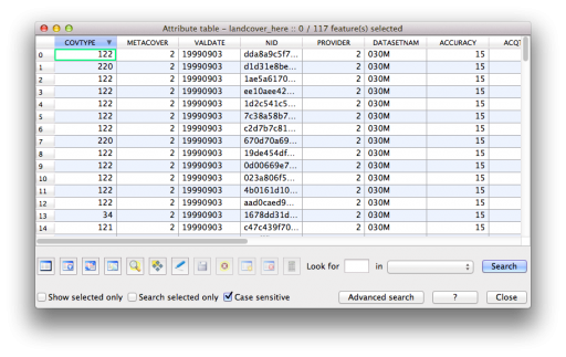
The fun stuff is hidden in the attribute table:

So the COVTYPE field is clearly holding something about the land cover type. But what?

GeoBase helpfully provide a PDF key and a style file — which only works with ArcGIS products. As a dedicated (okay, yes, cheap) user of Open GIS systems, this could not stand! So I dug through the Styled Layer Descriptor (SLD) format, and came up with style files (in both English & French) that work with QGIS: SLD_LCC2000-V-en_CSC2000-V-fr.zip.

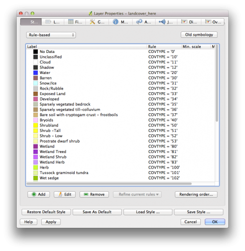
To use them with QGIS, open up the layer properties, and go to the Style tab. You want to use the New Symbology option, then Load Style … From here, you can open the SLD file (changing the file type from QGIS’s default QML to SLD), which should appear like this:

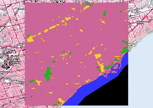
This makes the layer look much better:

Categories
GIS

Making weird composite shapes with Shapely

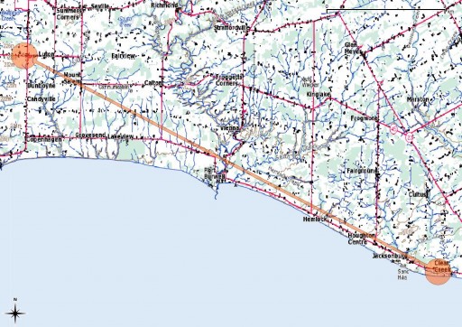
Let’s say you operate microwave radio links, and you want to see if you could build a link between, say, the huge comms tower at Clear Creek, ON and your tower just south of Aylmer. You know that Erie Shores Wind Farm is in the middle of the route. Do the 77m diameter turbines attenuate your signal to nothing?
This is a real issue I have to deal with every day, except in reverse: when I’m planning wind farms, I don’t want to be blocking existing licensed links. I use Spectrum Direct to find these links (and precisely two years ago, I showed you how to write Spectrum Direct data as CSV), but up until now I worked out affected zones (called “consultation zones”) by hand.

The Radio Advisory Board of Canada and the Canadian Wind Energy Association developed a joint protocol on sizing consultation zone for wind turbines, documented in the RABC CANWEA Guidelines. The one for a microwave link comprises:

  • A 1km buffer around the start and end points of the link;
  • A distance-, frequency- and wind-turbine diameter-specific path width between the points.

Here I’m only going to consider the 2D geometry of the path. Lots of people in the radio industry get paid money to do line-of-sight terrain analysis, and I’m ignoring this for now. All I’m doing here is using Python’s Shapely library to make the dumb-bell shaped buffer around the path and endpoints. I learned of Shapely from Erik Westra’s book Python Geospatial Development. Here’s some code that outputs pipe-separated well-known text that imports nicely into QGIS:

#!/usr/bin/python
# -*- coding: utf-8 -*-
# Calculate RABC/CanWEA Microwave Link Consultation Zone
# scruss - 2012-10-29

import pyproj
import shapely.geometry
from shapely.wkt import dumps

# hard-coded details (sorry)
startlat = 42.582892  # Clear Creek
startlong = -80.603875
endlat = 42.731776  # South Aylmer
endlong = -80.98768
frequency = 6e9  # 6 GHz
rotor = 77.0  # wtg rotor diameter, m

# calculate distance between points
g = pyproj.Geod(ellps='WGS84')
(az12, az21, dist) = g.inv(startlong, startlat, endlong, endlat)

# Width of microwave link fresnel zone
Lc = rotor + 52 * ((dist / 1000) / (frequency / 1e9)) ** 0.5

# calculate line string along path with segments <= 1 km
lonlats = g.npts(startlong, startlat, endlong, endlat,
                 1 + int(dist / 1000))

# npts doesn't include start/end points, so prepend/append them
lonlats.insert(0, (startlong, startlat))
lonlats.append((endlong, endlat))

# translate line string into projected coordinates
utms = []
srcp = pyproj.Proj(init='epsg:4326')  # WGS84
destp = pyproj.Proj(init='epsg:32617')  # WGS84 UTM Zone 17N
for (lon, lat) in lonlats:
    (utmx, utmy) = pyproj.transform(srcp, destp, lon, lat)
    utms.append((utmx, utmy))

# turn start and end points into Shapely point objects
startpt = shapely.geometry.Point(utms[0])
endpt = shapely.geometry.Point(utms[-1])

# draw a 1km buffer around start/end points
startb = startpt.buffer(1000)
endb = endpt.buffer(1000)

# convert microwave path to a Shapely LineString
path = shapely.geometry.LineString(utms)
pathb = path.buffer(Lc / 2) # buffer it to fresnel zone width

# join the buffers into one shape
zone = startb.union(pathb).union(endb)

# output the shape as well known text
print 'id|wkt'
print '|'.join(('1', dumps(zone)))

That little snippet creates the buffer in projected coordinates from two geographic coordinates as inputs. Grabbing the Erie Shores coordinates from OpenStreetMap and the USGS WMS, let’s see if the beam will pass:
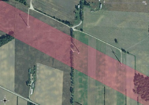
Uh, no. That’s three turbines in the path in that little section alone. Back to the drawing board.

Categories
Uncategorized

The Invisible City

Now you see it …

There’s not a whole lot north of North Bay. Highway 11 winds through some extensive geometry, but few habitations. Until something wonderful (and quite a bit wrong) happened at 46° 31′ 21″ N, 79° 33′ 9″ W on OpenStreetMap. A whole new town about 25 minutes out of North Bay sprung up overnight — and was as quickly deleted as mappers caught and reverted the vandalism.

Now you don’t.

The misguided mapper put quite a lot of work into this ephemeral town. It’s got urban rail, parklands, residential areas and more. You can see the detail on this large image of the town (650 KB PNG). If you want to play with the data, here’s a zipped OSM XML file of the area before it was reverted. But please, don’t re-upload it; OpenStreetMap should be for real features on the ground, and not for confusing map data consumers.

Thanks to Bootprint for noticing this, and to rw__ for reverting the edits.

Categories
GIS

Awesome USGS orthoimagery … in Canada?

Update, 2015: I don’t think this coverage works any more. The WMS data was carefully trimmed to the US border last time I looked.

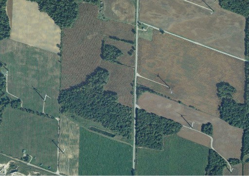
Detail of Erie Shores Wind Farm showing USGS orthophotos from WMS

I was trying to do some OpenStreetMap edits in rural southern Ontario, but the default Bing background aerial imagery is very poor. Clicking around in semi-plokta mode to find better images, I happened upon “OSM US USGS Large Scale Aerial Imagery”, which loaded up some beautiful and recent pictures. I guess that since we’re close to the border, the USGS doesn’t bother to trim its images too close.

Ian Dees, who admins the particular OSM server, confirmed that these are from The National Map‘s TNM_Large_Scale_Imagery service; thanks, Ian! These images are at least as good for my purposes as the SWOOP data — except not $50/km2, and without elaborate usage restrictions.

Categories
Uncategorized

Mephisto’s Oriental Mystery — solved!

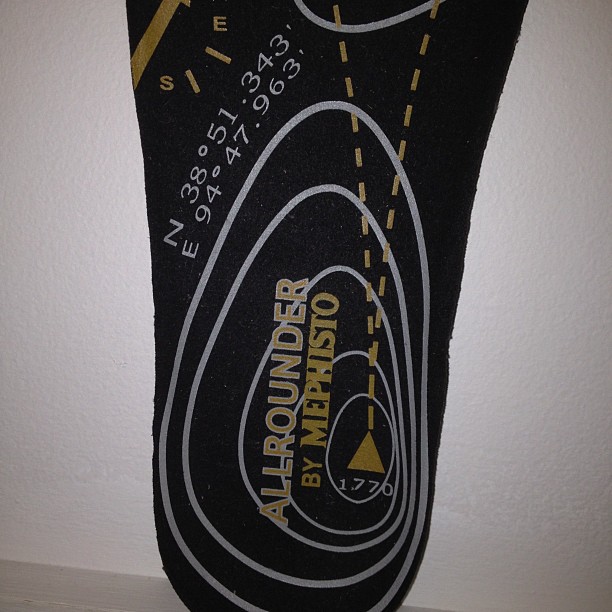
I bought a pair of Mephisto shoes today, and to go with their wayfaring imagery, the insoles are decked out with map-like symbols. Prominent is a map coordinate: N 38° 51.343′ E 94° 47.963′.

If you look at a map there, it’s a fairly empty mountainous place near the border of Qinghai and Gansu. It’s definitely not where the shoes are made, unless Mephisto have a stealth factory there.

There was something familiar about the coordinate, through. I thought I’d try flipping it to the western hemisphere:

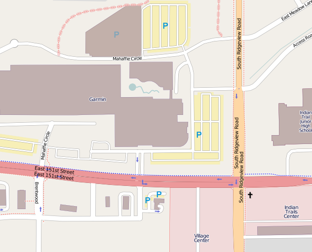
It’s the Garmin headquarters in Olathe, KS! Every Garmin GPS I’ve ever owned has had the HQ as a default waypoint. I’m guessing a designer at Mephisto was looking to add something legitimately mappy to the graphics, and picked up their satnav to pull out a coordinate. Guessing that Olathe isn’t a very mysterious, rugged destination, they flipped the hemisphere to give it more eastern promise.

Categories
GIS

Convert Manifold aux files to ESRI world files

The great thing about geospatial metadata standards is that there are so many to choose from. When slinging files about from user to user, it seems that mostly the ESRI stuff (well, the stuff we can pick apart, anyway) is used, plus some sedimentary layers deposited as good ideas from other systems. Commercial GIS systems are much less liberal, because all of them have the inertia of user investment.

Manifold does things its own way. Rather than using broadly standard prj or wld files, Manifold accompanies every exported file with an XML metafile in its own format. I get sent a lot of bitmaps from Manifold, and if I want to do more than view them on the screen, I need to convert the metadata.

Below is a small Awk program to convert a Manifold XML metadata file for a bitmap into an ESRI World file:

#!/bin/awk -f
# convert Manifold xml metadata to ESRI world file
# nb: this is not a general-purpose XML parser
# scruss - 20120508

BEGIN {
    indata = 0;
}

/<coordinateSystem>/ {
    indata = 1;			# in metadata section of file
}

/<\/coordinateSystem>/ {
    indata = 0;			# no longer in metadata
}

/</ && (indata == 1) {
    # build array of items
    sub(/<\/[^>]*>/, "", $0);	# remove end tag
    tagloc=match($0, /<[^>]*>/);
    if ((RSTART == 0) && (RLENGTH == -1)) { 
	# no match!
    }
    else {
	tag=substr($0, RSTART, RLENGTH);
	sub(/</, "", tag);	# remove < and > from tag
	sub(/>/, "", tag);
	value=substr($0, RSTART + RLENGTH); # value is rest of string
	params[tag] = value;
    }
}

END {
    # output six values for ESRI world file
    # all the "+ 0.0" stuff is just to force numeric output
    OFMT="%.10f";
    print params["localScaleX"] + 0.0;
    print params["rotationX"] + 0.0; # these will almost always be zero
    print params["rotationY"] + 0.0;
    print (params["localScaleY"] + 0.0) * -1.0; # negate Manifold value
    print params["localOffsetX"] + 0.0;
    print params["localOffsetY"] + 0.0;
}

Note that I’m doing what you’re supposed never to do — parse XML as if it were just some text format. If Manifold change their file format even slightly, this program will fail. The above seems to work on all the data I’ve thrown at it, although none of those test files included rotation terms. I don’t think I’ve ever actually seen a world file with rotation defined, so this may be a minor limitation.

Categories
GIS

geocoder.ca’s excellent database

Update, late 2017: Looks like geocoder.ca’s database hasn’t been updated since late 2015. The download link is still active, though.

geocoder.ca provides a crowdsourced postal code geocoder under the ODbL. You can download the database as CSV directly. Here’s a bash script to convert that text file into a (very large) point shapefile:

#!/bin/bash
# geocoder2shp.sh - convert geocoder.ca CSV to a shape file
# NB: input CSV is UTF-8; it is passed through unchanged
# Needs >= v1.7 of GDAL
# scruss - 2012/04/15

if [ ! -f Canada.csv.gz ]
then
    echo ""
    echo " " Download \"Canada.csv.gz\" into the current directory from
    echo "  " http://geocoder.ca/onetimedownload/Canada.csv.gz
    echo " " and try again.
    echo ""
    exit 1
fi

# make input file with header
echo PostalCode,Latitude,Longitude,City,Province > Canada2.csv
gunzip -c Canada.csv.gz >> Canada2.csv

# create GDAL VRT file
cat > Canada2.vrt <<EOF
<OGRVRTDataSource>
  <!-- note that OGRVRTLayer name must be basename of source file -->
  <OGRVRTLayer name="Canada2">
    <SrcDataSource>Canada2.csv</SrcDataSource>
    <GeometryType>wkbPoint</GeometryType>
    <LayerSRS>EPSG:4326</LayerSRS>
    <GeometryField encoding="PointFromColumns" x="Longitude" y="Latitude"/>
    <Field name="PostalCode" type="String" width="6" />
    <Field name="Latitude" type="Real" />
    <Field name="Longitude" type="Real" />
    <Field name="City" type="String" width="60" />
    <Field name="Province" type="String" width="2" />
  </OGRVRTLayer>
</OGRVRTDataSource>
EOF

# create shapefile
ogr2ogr PostalCodes.shp Canada2.vrt

# clean up
rm -f Canada2.csv	Canada2.vrt

Though the script is a bit Unix-centric, it’s just a simple list of instructions which could be run on any command line. What it does is add some headers to the geocoder.ca file, then sets up an OGR Virtual Format to convert the text into a fairly well-defined shapefile. When you use this shapefile, you should credit geocoder.ca as the ODbL requires.

Eek! geocoder.ca has been sued by Canada Post! (News responses: Michael Geist, Boing Boing, CBC) I’ve donated to defend this useful service.

Categories
GIS

Georeferencing QGIS output rasters

Some of the design packages I rely on use very crude GIS facilities. In fact, all they can support is a georeferenced raster as a background image, so it’s more of a rough map than GIS. It helps if these rasters are at a decent resolution, typically 1m/pixel or better.

A while back, I asked on the QGIS forum if the package could output high resolution georeferenced rasters. I received a rather terse response that no, it couldn’t (and I inferred from the tone that the poster thought that it shouldn’t, and I was wrong to want such a thing). I shelved the idea at the time.

After having to fix a lot of paths in a QGIS project file I’d moved to a new system, I noticed that all the map composer attributes are rather neatly defined in the XML file structure. Some messing around with Perl, XML::Simple and Data::Dumper::Simple, and I had a little script that would spit out an ESRI World File for the map composer raster defined in the project.

To run this, you have to create a project with just one Print Composer page, save the composed map as an image, save the project, then run the script like this:

./geoprint.pl project.qgs > image.pngw

There are some caveats:

  • This probably won’t work for projects with multiple print composers
  • It doesn’t quite get the scale right, but it’s within a pixel or so. I may not have corrected for image borders.

Though there’s some fairly hideous XML-mungeing in the code, what the script does is entirely trivial. If you feel you can use it, good; if you feel you can improve it, be my guest.

#!/usr/bin/perl -w
# geoprint - georef a QGIS output image by creating a world file
# one arg: qgis project file (xml)
# $Id: geoprint.pl,v 1.3 2012/04/06 03:32:01 scruss Exp $

use strict;
use XML::Simple;
use constant MM_PER_INCH =&amp;gt; 25.4;

my $qgis = $ARGV[0];
die &amp;quot;$qgis must exist\n&amp;quot; unless ( -f $qgis );

my $q = XMLin($qgis) or die &amp;quot;$!\n&amp;quot;;
my %composer = %{ $q-&amp;gt;{Composer} };
my $image_width =
  int( $composer{Composition}-&amp;gt;{paperWidth} *
    $composer{Composition}-&amp;gt;{printResolution} /
    MM_PER_INCH );
my $image_height =
  int( $composer{Composition}-&amp;gt;{paperHeight} *
    $composer{Composition}-&amp;gt;{printResolution} /
    MM_PER_INCH );

# we need xpixelsize, ypixelsize, ulx and uly
my $xpixelsize =
  ( $composer{ComposerMap}-&amp;gt;{Extent}-&amp;gt;{xmax} -
    $composer{ComposerMap}-&amp;gt;{Extent}-&amp;gt;{xmin} ) /
  int( $composer{ComposerMap}-&amp;gt;{ComposerItem}-&amp;gt;{width} *
    $composer{Composition}-&amp;gt;{printResolution} /
    MM_PER_INCH );
my $ypixelsize =
  -1.0 *
  ( $composer{ComposerMap}-&amp;gt;{Extent}-&amp;gt;{ymax} -
    $composer{ComposerMap}-&amp;gt;{Extent}-&amp;gt;{ymin} ) /
  int( $composer{ComposerMap}-&amp;gt;{ComposerItem}-&amp;gt;{height} *
    $composer{Composition}-&amp;gt;{printResolution} /
    MM_PER_INCH );
my $ulx =
  $composer{ComposerMap}-&amp;gt;{Extent}-&amp;gt;{xmin} -
  $xpixelsize *
  int( $composer{ComposerMap}-&amp;gt;{ComposerItem}-&amp;gt;{x} *
    $composer{Composition}-&amp;gt;{printResolution} /
    MM_PER_INCH ) - $xpixelsize;
my $uly =
  $composer{ComposerMap}-&amp;gt;{Extent}-&amp;gt;{ymax} -
  $ypixelsize *
  int( $composer{ComposerMap}-&amp;gt;{ComposerItem}-&amp;gt;{y} *
    $composer{Composition}-&amp;gt;{printResolution} /
    MM_PER_INCH ) - $ypixelsize;

printf( &amp;quot;%.12f\n%.12f\n%.12f\n%.12f\n%.12f\n%.12f\n&amp;quot;,
  $xpixelsize, 0.0, 0.0, $ypixelsize, $ulx, $uly );

# FIXME? pixel scale seems a tiny bit off - allow for border?
exit;
Categories
Uncategorized

map nap

At the Toronto Hack Weekend, Henk Hoff presented Richard with a very nice Soft Cities – Midnight Commander Blanket. Soft! Mappy!!