Generated using ptrv/gpx2spatialite, rendered in QGIS as lines with 75% transparency.
Generated using ptrv/gpx2spatialite, rendered in QGIS as lines with 75% transparency.
 @MaptimeTO asked me to summarize the brief talk I gave last week at Maptime Toronto on making maps from the Technical and Administrative Frequency List (TAFL) radio database. It was mostly taken from posts on this blog, but here goes:
Today, I’m going to describe how I get fairly accurate buffer distances over a really large area.
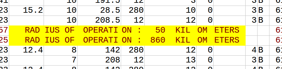
But first, I’m going to send a huge look of disapproval (![]() ) to Norway. It’s not for getting all of the oil and finding a really mature way of dealing with it, and it’s not for the anti-personnel foods (rancid fish in a can, salt liquorice, sticky brown cheese …) either. It’s for this:
) to Norway. It’s not for getting all of the oil and finding a really mature way of dealing with it, and it’s not for the anti-personnel foods (rancid fish in a can, salt liquorice, sticky brown cheese …) either. It’s for this:
The rest of the world is perfectly fine with having their countries split across Universal Transverse Mercator zones, but not Norway. “Och, my wee fjords…” they whined, and we gave them a whole special wiggle in their UTM zone. Had it not been for Norway’s preciousness, GIS folks the work over could’ve just worked out their UTM zone from a simple calculation, as every other zone is just 6° of longitude wide.
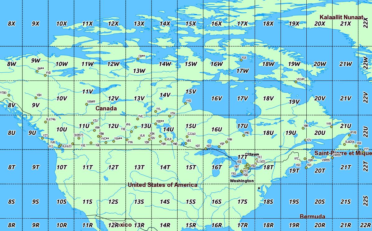
Canada has no such qualms. In a big country (dreams stay with you …), we have a lot of UTM zones:
 We’re in zones 8–22, which is great if you’re working in geographic coordinates. If you’re unlucky enough to have to apply distance buffers over a long distance, the Earth is inconveniently un-flat, and accuracy falls apart.
What we can do, though, is transform a geographic coordinate into a projected one, apply a buffer distance, then transform back to geographic again. UTM zones are quite good for this, and if it weren’t for bloody Norway, it would be a trivial process. So first, we need a source of UTM grid data.
Well, the Global UTM Zones Grid from EPDI looks right, and it’s CC BY-NC-SA licensed. But it’s a bit busy with all the grid squares:
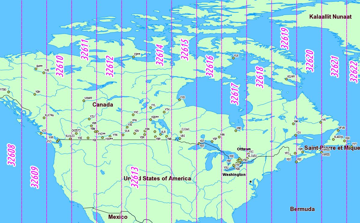
 What’s more, there’s no explicit way of getting the numeric zone out of the CODE field (used as labels above). We need to munge this a bit. In a piece of gross data-mangling, I’m using an awk (think: full beard and pork chops) script to process a GeoJSON (all ironic facial hair and artisanal charcuterie) dump of the shape file. I’m not content to just return the zone number; I’m turning it into the EPSG WGS84 SRID of the zone, a 5-digit number understood by proj.4:
32hzz
where:
I live in Zone 17 North, so my SRID is 32617.
Here’s the code to do it: zones_add_epsg-awk (which you’ll likely have to rename/fix permissions on). To use it:
And, lo!
 So we can now load this wgs84utm shapefile as a table in SpatiaLite. If you wanted to find the zone for the CN Tower (hint: it’s the same as me), you could run:
select EPSGSRID from wgs84utm where within(GeomFromText('POINT(-79.3869585 43.6425361)',4326), geom);
which returns ‘32617’, as expected.
(I have to admit, I was amazed when this next bit worked.)
Let’s say we have to identify all the VOR stations in Canada, and draw a 25 km exclusion buffer around them (hey, someone might want to …). VOR stations can be queried from TAFL using the following criteria:
This can be coded as:
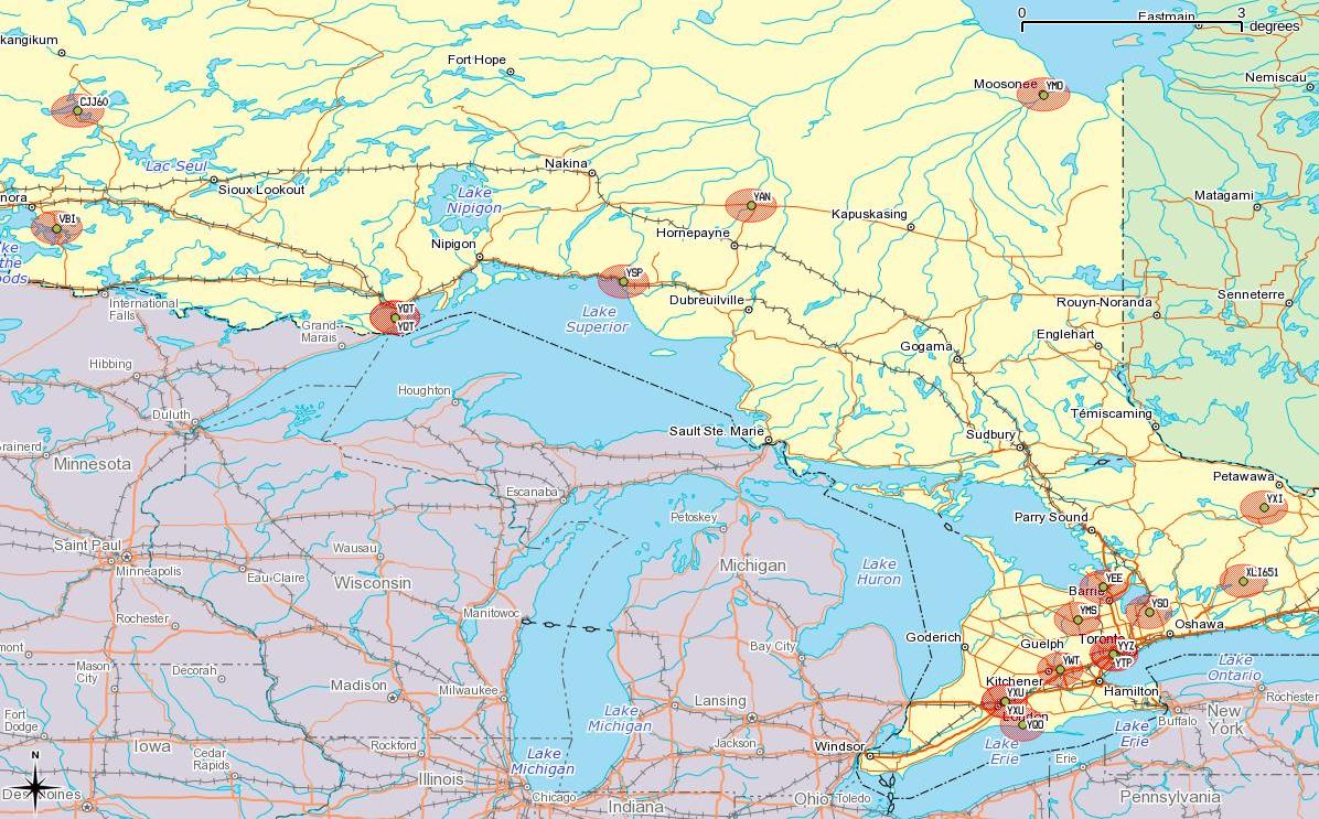
SELECT * FROM tafl WHERE licensee LIKE 'NAV CANADA%' AND tx >= 108 AND tx <= 117.96 AND location LIKE '%VOR%';which returns a list of 67 stations, from VYT80 on Mount Macintyre, YT to YYT St Johns, NL. We can use this, along with the UTM zone query above, to make beautiful, beautiful circles:
SELECT tafl.PK_ROWID, tafl.tx, tafl.location, tafl.callsign, Transform (Buffer ( Transform ( tafl.geom, wgs84utm.epsgsrid ), 25000 ) , 4326 ) AS bgeom FROM tafl, wgs84utm WHERE tafl.licensee LIKE 'NAV CANADA%' AND tafl.tx >= 108 AND tafl.tx < 117.96 AND tafl.location LIKE '%VOR%' AND Within( tafl.geom, wgs84utm.geom );Ta-da!
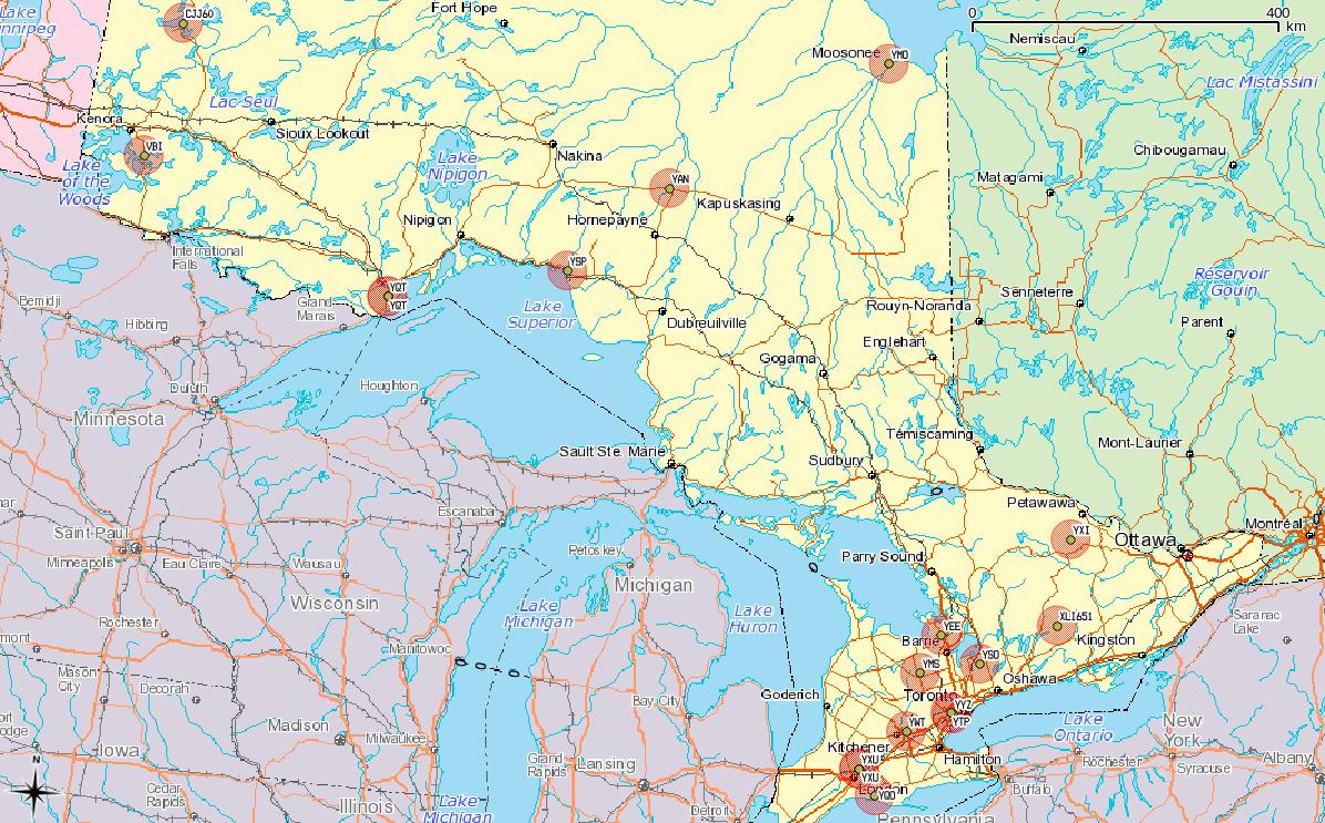
Yes, they look oval; don’t forget that geographic coordinates don’t maintain rectilinearity. Transformed to UTM, they look much more circular:
Update, 2017: TAFL now seems to be completely dead, and Spectrum Management System has replaced it. None of the records appear to be open data, and the search environment seems — if this is actually possible — slower and less feature-filled than in 2013.
Update, 2013-08-13: Looks like most of the summary pages for these data sets have been pulled from data.gc.ca; they’re 404ing. The data, current at the beginning of this month, can still be found at these URLs:
I build wind farms. You knew that, right? One of the things you have to take into account in planning a wind farm is existing radio infrastructure: cell towers, microwave links, the (now-increasingly-rare) terrestrial television reception.
I’ve previously written on how to make the oddly blobby shape files to avoid microwave links. But finding the locations of radio transmitters in Canada is tricky, despite there being two ways of doing it:
So searching for links is far from obvious, and it’s not like wireless operators do anything conventional like register their links on the title of the properties they cross … so these databases are it, and we must work with them.
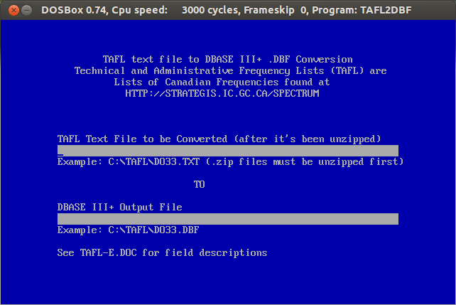
The good things is that TAFL is now Open Data, defined by a reasonable Open Government Licence, and available on the data.gc.ca website. Unfortunately, the official Industry Canada tool to process and query these files, is a little, uh, behind the times:Yes, it’s an MS-DOS exe. It spits out DBase III Files. It won’t run on Windows 7 or 8. It will run on DOSBox, but it’s rather slow, and fails on bigger files.
That’s why I wrote taflmunge. It currently does one thing properly, and another kinda-sorta:
taflmunge runs anywhere SpatiaLite does. I’ve tested it on Linux and Windows 7. It’s just a SQL script, so no additional glue language required. The database can be queried on anything that supports SQLite, but for real spatial cleverness, needs SpatiaLite loaded. Full instructions are in the taflmunge / README.md.
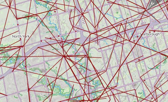
TAFL is clearly maintained by licensees, as the data can be a bit “vernacular”. Take, for example, a tower near me:
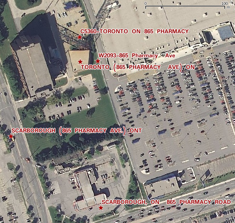
The tower is near the top of the image, but the database entries are spread out by several hundred meters. It’s the best we’ve got to work with.
Ultimately, I’d like to keep this maintained (the Open Data TAFL files are updated monthly), and host it in a nice WebGIS that would allow querying by location, frequency, call sign, operator, … But that’s for later. For now, I’ll stick with refining it locally, and I hope that someone will find it useful.
Mark asked: What kind of GIS software are you using?
Well, since you asked:-
All of the above are free. I’m doing this because I want to learn. Asking elsewhere hasn’t turned up anything useful.
Now I’ve sorted out formatting the labels and scraping the data, I should be almost ready to produce a pretty map.
Well, almost. The DBF component of a shapefile seems somewhat resistant to adding a column, and SQLite doesn’t seem very happy with its ALTER TABLE ADD COLUMN ... syntax.
As usual, I needed to create the database table from the shapefile. I’m not bothered about CRS, so I used -1.
.read init_spatialite-2.3.sql ASCII

.loadshp TCL3_ICITW Wards CP1252 -1

alter table wards add column candidates integer
I had mixed success getting data to load into this new column. So I improvised.
!!! WARNING: EGREGIOUS MISUSE OF DATA FOLLOWS !!!
(Sensitive readers are advised to look away)
There’s a seeming unused numeric column SHAPE_LEN in the table. As my new candidates column was coming up with occasional nulls, I cheated:
UPDATE Wards set shape_len=3 where scode_name="1"

UPDATE Wards set shape_len=1 where scode_name="2"

UPDATE Wards set shape_len=0 where scode_name="3"

...

UPDATE Wards set shape_len=3 where scode_name="44";
I then added SHAPE_LEN as the label, and defined a range based colour gradient for the wards in QGIS’s layer properties:
 And this is how it looks:
 Another partial success, as Professor Piehead would say.
My post diary of a geonumpty to my main blog is really what got me started thinking about abstract geographic data. In it, I (with a lot of external help) develop queries to count points in areas with the same owner, and find points outside properties.
 For reasons that are not particularly clear, the Toronto.ca|Open data is in two different coordinate reference systems (CRS), MTM 3 Degree Zone 10, NAD27 (EPSG 2019) and UTM 6 Degree Zone 17N NAD27 (EPSG 26717). This confuses QGIS even if you’ve input the proper SRIDs into SpatiaLite. The image above shows two apparent Torontos, one in each of the CRSs.
What you have to do is go to to the Project Properties, select the Coordinate Reference System (CRS) tab, and “Enable ‘on the fly’ CRS transformation”. This will line those city layers right back up.
 Once we do that, things align as they should. Here’s my neighbourhood, with its parks
 But things are still off if you’re querying the SQL directly:
select Distance(Parks.geometry, Neighbourhoods.geometry)/1000
 as Distance_km
 from Parks, Neighbourhoods
 where Parks.name='CORVETTE PARK'
 and Neighbourhoods.hood='Kennedy Park'
which returns a distance of over 314 km. That’s not right.
So we need to transform the geometries to the same CRS.
!!! NB: I might be doing the next bit wrong. CRS transformation is subtle. I’m not, particularly.
The OGR Simple Feature Library is your friend. It can convert pretty much any geo format to another, and can transform coordinates between systems. In exchange for this power, it wants your soul is rather complex.
I’ve chosen to use NAD83(CSRS) / UTM zone 17N (EPSG 2958) for my Toronto maps. It’s fairly accurate over the whole city area. To convert the Parks and Neighbourhoods shape files:
ogr2ogr -s_srs EPSG:2019 -t_srs EPSG:2958 dest/2958/parks/TCL3_UPARK.shp src/2019/parks/TCL3_UPARK.shp
ogr2ogr -s_srs EPSG:26717 -t_srs EPSG:2958 dest/2958/neighbourhoods/Neighbourhoods.shp src/26717/neighbourhoods/Neighbourhoods.shp
Note that it wants the destination file first, then the source. Haven’t seen that order since PIP under CPM/2.2. I was also a bit nerdly, and arranged the files in directories by SRID:
src/2019/address-points

src/2019/business-improvement-areas

src/2019/city-wards

src/2019/parks

src/2019/solid-waste-management-districts

src/2019/toronto-centreline

src/26717/food-banks

src/26717/neighbourhoods

src/26717/places-of-worship

src/26717/priority-invest-neighbourhoods

src/26717/rent-bank-zones

src/26717/rent-banks

src/26717/transit-city

dest/2958/address-points

dest/2958/business-improvement-areas

dest/2958/city-wards

dest/2958/food-banks

dest/2958/neighbourhoods

dest/2958/parks

dest/2958/places-of-worship

dest/2958/priority-invest-neighbourhoods

dest/2958/rent-bank-zones

dest/2958/rent-banks

dest/2958/solid-waste-management-districts

dest/2958/toronto-centreline

dest/2958/transit-city
If we load the transformed shapefiles into Spatialite, and run that query again, it comes out with the correct distance: 0.0 km, as Corvette Park is in the Kennedy Park Neighbourhood.
Now we can run a proper query: what parks are in Kennedy Park, and what are their areas?
select tp.name, round(Area(tp.geometry)/10000,1) as Area_ha
 from Parks as tp, Neighbourhoods as tn
where tn.hood='Kennedy Park'
 and within(tp.geometry, tn.geometry)
order by Area_ha
| NAME | Area_ha |
|---|---|
| MAYWOOD TOT LOT | 0.7 |
| KITCHENER PARK | 0.8 |
| GLEN SHEPPARD PARK | 1.0 |
| GREYSTONE PARK | 1.1 |
| CORVETTE PARK | 2.5 |
| MID-SCARBOROUGH C.C. & ARENA | 2.9 |
| FARLINGER RAVINE | 2.9 |
(note how I sneakily used the round() function to avoid too many decimal places?)
Me and Catherine are quite partial to libraries. I’m going to use the address points database we made yesterday to find the libraries within 2km of a given address. It’s not a very useful query, but it shows the very basics of searching by distance.
I’m going to use the address from yesterday, 789 Yonge St. The fields I’m interested in are:
I’m also going to use a calculated field for the distance to make the query shorter. Since my map units are metres, calculating Distance(…)/1000 will return kilometres. So:
select t2.name, t2.address, t2.lf_name,
distance( t1.geometry, t2.geometry ) / 1000 as
 Distance_km
from TCL3_ADDRESS_POINT as t1,
 TCL3_ADDRESS_POINT as t2
where t1.address = 789 and t1.lf_name =
 'YONGE ST' and t2.fcode_desc = 'Library' and
 distance_km < 2
 order by distance_km
Note I’m using two instances of the same table; one for the source address (t1), and the other for the destinations (t2). The results I get are:
| NAME | ADDRESS | LF_NAME | Distance_km |
|---|---|---|---|
| Toronto Reference | 789 | YONGE ST | 0.0 |
| Yorkville | 22 | YORKVILLE AVE | 0.161394052244849 |
| 130 | ST GEORGE ST | 1.2973836702297 | |
| Spadina Road | 10 | SPADINA RD | 1.52482151385834 |
| 252 | MC CAUL ST | 1.58040842489387 | |
| 40 | ST GEORGE ST | 1.59417399071161 | |
| Lillian H.Smith Library | 239 | COLLEGE ST | 1.81606690760918 |
| 265 | GERRARD ST E | 1.86262658418202 | |
| Parliament | 269 | GERRARD ST E | 1.87733631488281 |
| Deer Park | 40 | ST CLAIR AVE E | 1.9224871094566 |
There’s one at zero distance, because 789 Yonge St is a library, so the search finds itself. Try any other address, and you wouldn’t get the zero. I’m pretty sure the 14 decimal places is overkill.
I see that some of the libraries don’t have names. I’m pretty sure that the St George St ones are the UofT Library, and the McCaul St one is OCAD‘s, but the others, I can’t tell.