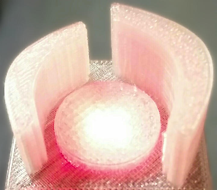

Based on Selasi Dorkenoo and Claus Rinner’s presentation at Toronto #Maptime – 3D Printing Demo. More later.
Based on Selasi Dorkenoo and Claus Rinner’s presentation at Toronto #Maptime – 3D Printing Demo. More later.
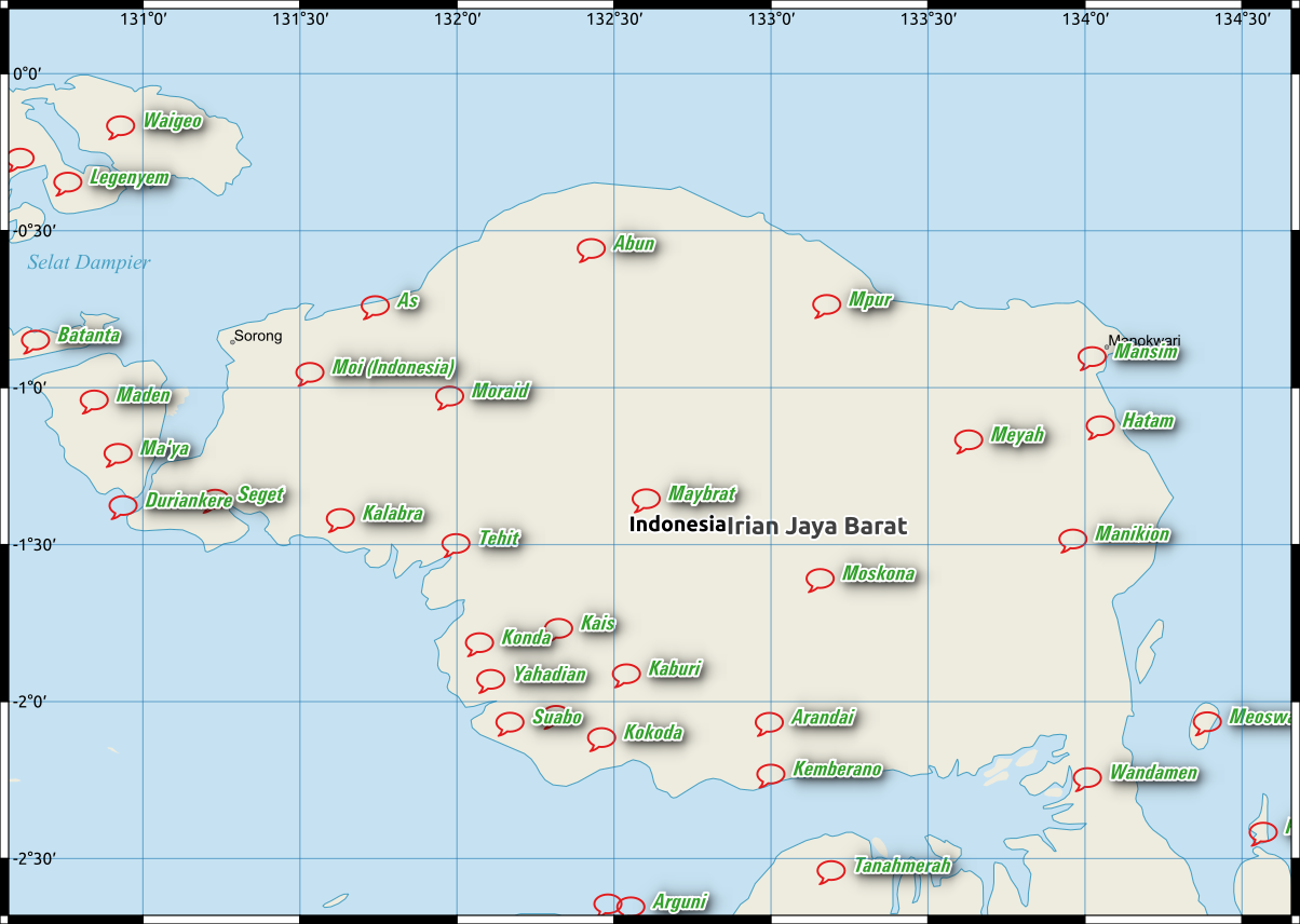
Map background: Natural Earth (public domain)
Language point data: Glottolog (licence: Creative Commons — Attribution-ShareAlike 3.0 Unported — CC BY-SA 3.0)
Map markers: font: Overpass (licence: SIL OFL/LGPL), character: 💬 — U+1F4AC SPEECH BALLOON.
Label font: U001Con Italic (foundry: URW++, licence: AFPL)
for more details, please see:
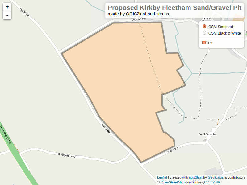
Minerals and waste joint plan consultation – North Yorkshire County Council http://northyorks.gov.uk/article/23999/Minerals-and-waste-joint-plan-consultation
Outline traced from http://northyorks.gov.uk/media/30250/Supplementary-sites-consultation—January-2015/pdf/Supplementary_sites_Consultation-_Web_Version.pdf
Update: After reading Anita’s article about Publishing interactive web maps using QGIS, I had to try the QGIS2leaf plugin. And lo! It works:
Joshua Frazier’s great tutorial Let’s make some web maps using Leaflet.js! for Maptime Toronto was a huge help in getting me started with Leaflet. Thanks, Joshua!
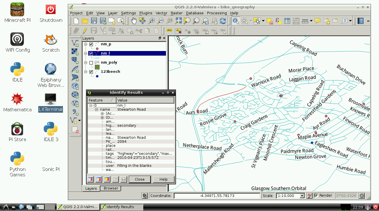
Growing up in a small country, I assumed the whole world used metric grid map coordinates. I mean, why would anyone bother with those tedious latitudes and longitudes when you could have your location defined by something as neat as NS539555?
The tidy, militaristic Ordnance Survey came up with the National Grid reference system, where large grid squares were given letters, and the rest of the reference was given numerically. Wikipedia gives a better graphical explanation than I could:

During WW2, the UK war office extended this system across most of Europe. Since most European countries didn’t use exactly the same Transverse Mercator projection as the UK did, a number of existing mapping systems were pressed into use, but using the same interleaved alphanumeric format as the OS grid reference.
The reference site for these systems is Thierry Arsicaud’s excellent Notes on the “Modified British System” used on the European Theatre of Operations during the WWII. Thierry, however, wasn’t trying to use these historical map references in a GIS, so his work needs a little massage to get to be used with QGIS.
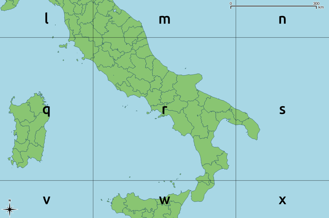
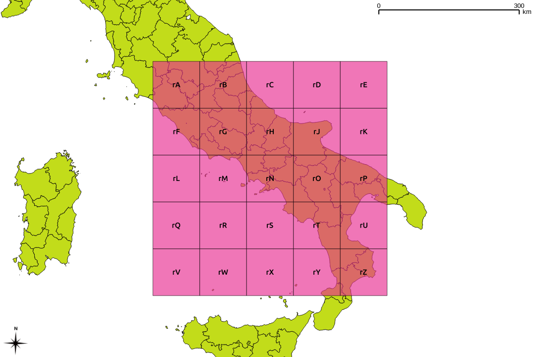
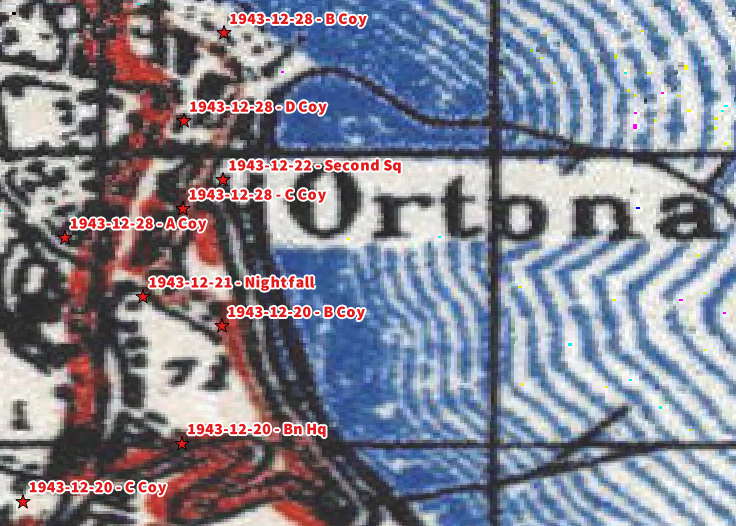
In this example, I’m going to concentrate on the South Italy zone, as that’s where I was asked to look at some war diaries from 1943. The system is similar to the OS grid, but the main difference is that the major grid reference is often given in lower case. So RN in OSGB would most often be denoted rN in the Modified British system. Both would refer to a 100 km square at (700, 700) km from the origin. (The exceedingly nitpicky might point out that RN is never used in the UK as it’s somewhere in the Atlantic, west of Ireland. To them, I say: Well, bless your heart …)
The key to both the OSGB grid and the Modified British system is a 2500 × 2500 km square, split into 25 500 km squares, and given a letter, a … z with i excluded:

Each letter encodes both an easting and a northing; so r is (500000, 500000). About the easiest way to unpack this encoding is through a simple string lookup:
result = SEARCH(letter, "VWXYZQRSTULMNOPFGHJKABCDE")-1
easting = result MOD 5
northing = INT(result / 5)
where SEARCH is a function which returns the position of a letter in a string (so SEARCH(“V”, “VWXYZ…”) returns 1).
When applied as per the GSGS South Italy system, you get something like this:
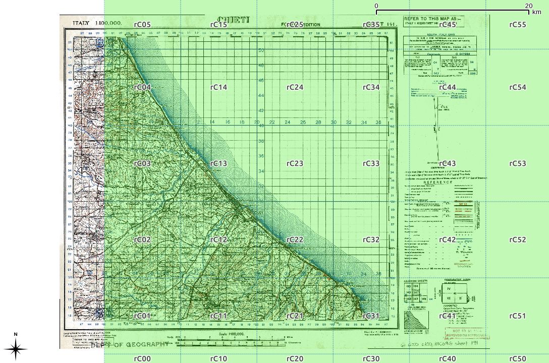
These major grid squares are in turn split into 25 minor squares of 100 km side:

Or overlaid on a map:
For grid references of higher precision, a series of numbers is appended. There should always be an even count of these numbers, for reasons which should become clear soon. Here is the rC square, split into 10 km references:

These two digit references are about the shortest/least precise you might ever see. Overlaid on an appropriate sheet from the McMaster archive WWII Topographic Map Series (which are CC BY-NC; for which, many thanks), you get:
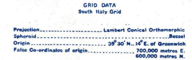
The actual projection details are given on each map:
We can turn this into a PROJ.4 definition:
Projection - Lambert Conical Orthomorphic  →    +proj=lcc
Ellipsoid: Bessel 1841                     →    +ellps=bessel
False Easting : 700000                     →    +x_0=700000
False Northing : 600000                    →    +y_0=600000
Central Meridian : 14.0°                   →    +lon_0=14
Central Parallel : 39.5°                   →    +lat_0=39.5 +lat_1=39.5
Scale Factor : 0.99906                     →    +k_0=0.99906
                       (other proj.4 terms)     +units=m +no_defs
or in one line,
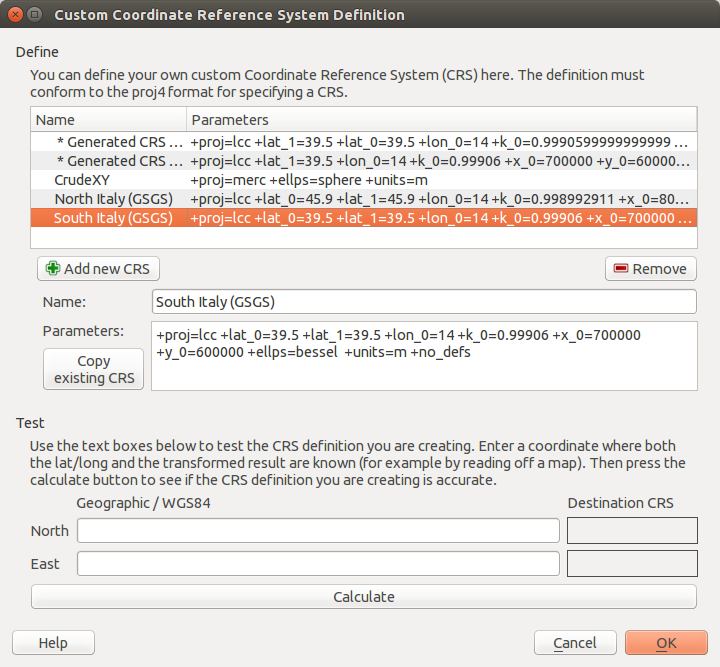
+proj=lcc +lat_0=39.5 +lat_1=39.5 +lon_0=14 +k_0=0.99906 +x_0=700000 +y_0=600000 +ellps=bessel +units=m +no_defs
In QGIS, you can plug those values into the Custom CRS manager, and you will be able to work in these antiquated coordinate systems with ease:
I haven’t yet quite managed to work out some of the other GSGS coordinate systems. My work on North Italy is a stubborn 100 km off true, for no well-defined reason. I haven’t managed to work out unpicking alphanumeric grid references into geometries automatically, either. These will come later.
Finally, some of the coordinates you might see might not meet these specifications. In the limited survey I’ve done, I’ve noted:
Huge thanks to Thierry Arsicaud, both for the great reference website, and also for the e-mail correspondence helping explain the parameters for the GSGS Italy South system. Props too to the Geographic Information Systems Stack Exchange folks for help with working out the proj.4 settings.
Hey! This is really old! The current version of Raspbian has QGIS 2.4 included in the repository. Just install that. It won’t run very fast on single-core Raspberry Pis, though.
sudo vi /etc/apt/sources.list # or use your favourite editorwheezy to jessiesudo apt-get updatesudo apt-get upgrade # this will take a long time, with occasional user promptssudo apt-get dist-upgrade # this will take a very long time …sudo apt-get install gdal-bin qgisThis will install QGIS 2.2. It’s a bit slow for general use, but it does work …
(modified from my gis.stackexchange answer: linux – GDAL and QGIS Raspberry Pi. Mainly just so I would have a place to put the image.)

Generated using ptrv/gpx2spatialite, rendered in QGIS as lines with 75% transparency.

André shows you how to add the OSGB New Popular Edition maps of England as a TMS layer in QGIS.
Today, I’m going to describe how I get fairly accurate buffer distances over a really large area.
But first, I’m going to send a huge look of disapproval (![]() ) to Norway. It’s not for getting all of the oil and finding a really mature way of dealing with it, and it’s not for the anti-personnel foods (rancid fish in a can, salt liquorice, sticky brown cheese …) either. It’s for this:
) to Norway. It’s not for getting all of the oil and finding a really mature way of dealing with it, and it’s not for the anti-personnel foods (rancid fish in a can, salt liquorice, sticky brown cheese …) either. It’s for this:
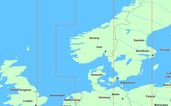
The rest of the world is perfectly fine with having their countries split across Universal Transverse Mercator zones, but not Norway. “Och, my wee fjords…” they whined, and we gave them a whole special wiggle in their UTM zone. Had it not been for Norway’s preciousness, GIS folks the work over could’ve just worked out their UTM zone from a simple calculation, as every other zone is just 6° of longitude wide.
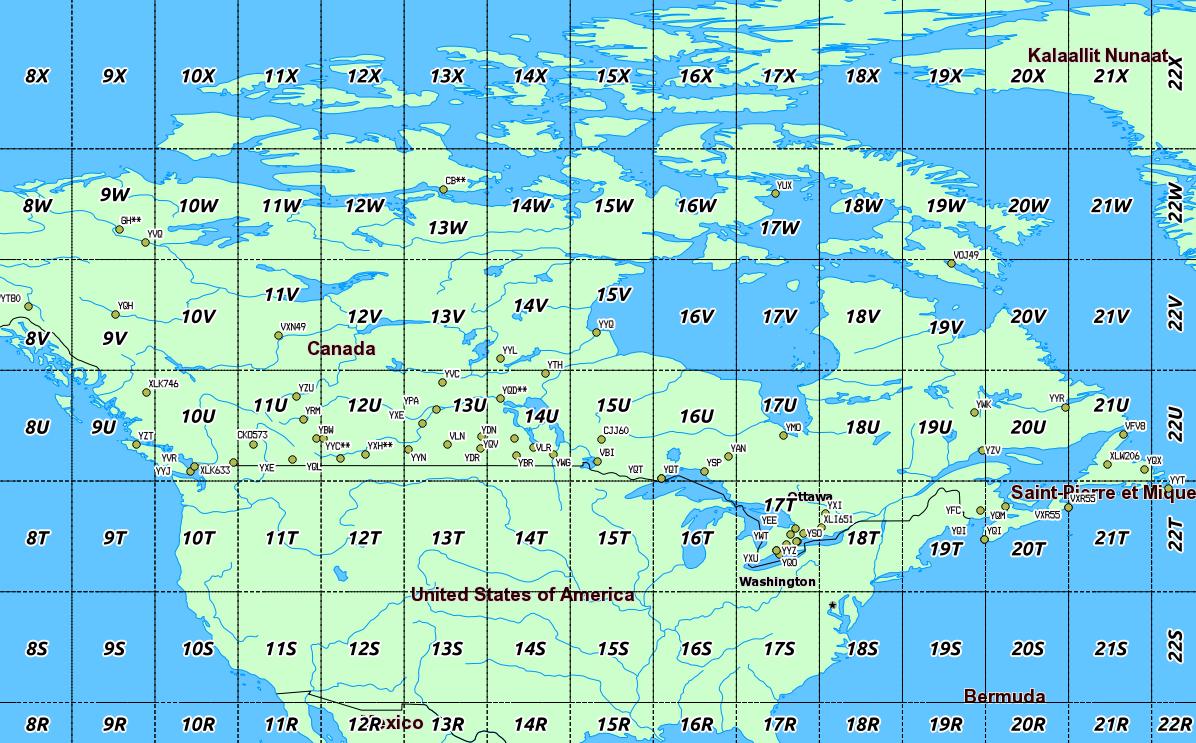
Canada has no such qualms. In a big country (dreams stay with you …), we have a lot of UTM zones:
 We’re in zones 8–22, which is great if you’re working in geographic coordinates. If you’re unlucky enough to have to apply distance buffers over a long distance, the Earth is inconveniently un-flat, and accuracy falls apart.
What we can do, though, is transform a geographic coordinate into a projected one, apply a buffer distance, then transform back to geographic again. UTM zones are quite good for this, and if it weren’t for bloody Norway, it would be a trivial process. So first, we need a source of UTM grid data.
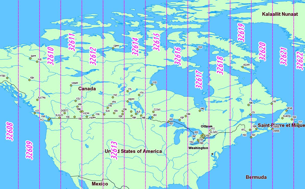
Well, the Global UTM Zones Grid from EPDI looks right, and it’s CC BY-NC-SA licensed. But it’s a bit busy with all the grid squares:
 What’s more, there’s no explicit way of getting the numeric zone out of the CODE field (used as labels above). We need to munge this a bit. In a piece of gross data-mangling, I’m using an awk (think: full beard and pork chops) script to process a GeoJSON (all ironic facial hair and artisanal charcuterie) dump of the shape file. I’m not content to just return the zone number; I’m turning it into the EPSG WGS84 SRID of the zone, a 5-digit number understood by proj.4:
32hzz
where:
I live in Zone 17 North, so my SRID is 32617.
Here’s the code to do it: zones_add_epsg-awk (which you’ll likely have to rename/fix permissions on). To use it:
And, lo!
 So we can now load this wgs84utm shapefile as a table in SpatiaLite. If you wanted to find the zone for the CN Tower (hint: it’s the same as me), you could run:
select EPSGSRID from wgs84utm where within(GeomFromText('POINT(-79.3869585 43.6425361)',4326), geom);
which returns ‘32617’, as expected.
(I have to admit, I was amazed when this next bit worked.)
Let’s say we have to identify all the VOR stations in Canada, and draw a 25 km exclusion buffer around them (hey, someone might want to …). VOR stations can be queried from TAFL using the following criteria:
This can be coded as:
SELECT * FROM tafl WHERE licensee LIKE 'NAV CANADA%' AND tx >= 108 AND tx <= 117.96 AND location LIKE '%VOR%';which returns a list of 67 stations, from VYT80 on Mount Macintyre, YT to YYT St Johns, NL. We can use this, along with the UTM zone query above, to make beautiful, beautiful circles:
SELECT tafl.PK_ROWID, tafl.tx, tafl.location, tafl.callsign, Transform (Buffer ( Transform ( tafl.geom, wgs84utm.epsgsrid ), 25000 ) , 4326 ) AS bgeom FROM tafl, wgs84utm WHERE tafl.licensee LIKE 'NAV CANADA%' AND tafl.tx >= 108 AND tafl.tx < 117.96 AND tafl.location LIKE '%VOR%' AND Within( tafl.geom, wgs84utm.geom );Ta-da!
Yes, they look oval; don’t forget that geographic coordinates don’t maintain rectilinearity. Transformed to UTM, they look much more circular:
ClickFu is dead in QGIS 3. Please try to forget how useful it was. nextgis / clickfu appears to be an updated version, but it has old QT dependencies and no longer works either.
Since QGIS 1.8 took the rather boneheaded move of hiding all the plugin sources except the official one, here’s how to get the other repositories back:
Now you can add all the plugins!
ClickFu is kind of magic. It allows you to choose an online map service, click anywhere on your GIS viewport, and the correct location link opens in your browser. Very handy for sharing locations with people who don’t have a GIS setup. It properly takes coordinate reference systems into account, too, so no messing about with datum shifts and the like.
Another plugin that hasn’t made it to the official repo is Luiz Motta’s Zip Layers. It still lurks at http://pyqgis.org/repo/contributed.
Click Fu runs just fun under QGIS 2.2 – as long as you remember to delete any pre-2.0 versions and then reinstall.