Categories
GIS

Awesome USGS orthoimagery … in Canada?

Update, 2015: I don’t think this coverage works any more. The WMS data was carefully trimmed to the US border last time I looked.

Detail of Erie Shores Wind Farm showing USGS orthophotos from WMS

I was trying to do some OpenStreetMap edits in rural southern Ontario, but the default Bing background aerial imagery is very poor. Clicking around in semi-plokta mode to find better images, I happened upon “OSM US USGS Large Scale Aerial Imagery”, which loaded up some beautiful and recent pictures. I guess that since we’re close to the border, the USGS doesn’t bother to trim its images too close.

Ian Dees, who admins the particular OSM server, confirmed that these are from The National Map‘s TNM_Large_Scale_Imagery service; thanks, Ian! These images are at least as good for my purposes as the SWOOP data — except not $50/km2, and without elaborate usage restrictions.

Categories
GIS

Convert Manifold aux files to ESRI world files

The great thing about geospatial metadata standards is that there are so many to choose from. When slinging files about from user to user, it seems that mostly the ESRI stuff (well, the stuff we can pick apart, anyway) is used, plus some sedimentary layers deposited as good ideas from other systems. Commercial GIS systems are much less liberal, because all of them have the inertia of user investment.

Manifold does things its own way. Rather than using broadly standard prj or wld files, Manifold accompanies every exported file with an XML metafile in its own format. I get sent a lot of bitmaps from Manifold, and if I want to do more than view them on the screen, I need to convert the metadata.

Below is a small Awk program to convert a Manifold XML metadata file for a bitmap into an ESRI World file:

#!/bin/awk -f
# convert Manifold xml metadata to ESRI world file
# nb: this is not a general-purpose XML parser
# scruss - 20120508

BEGIN {
    indata = 0;
}

/<coordinateSystem>/ {
    indata = 1;			# in metadata section of file
}

/<\/coordinateSystem>/ {
    indata = 0;			# no longer in metadata
}

/</ && (indata == 1) {
    # build array of items
    sub(/<\/[^>]*>/, "", $0);	# remove end tag
    tagloc=match($0, /<[^>]*>/);
    if ((RSTART == 0) && (RLENGTH == -1)) { 
	# no match!
    }
    else {
	tag=substr($0, RSTART, RLENGTH);
	sub(/</, "", tag);	# remove < and > from tag
	sub(/>/, "", tag);
	value=substr($0, RSTART + RLENGTH); # value is rest of string
	params[tag] = value;
    }
}

END {
    # output six values for ESRI world file
    # all the "+ 0.0" stuff is just to force numeric output
    OFMT="%.10f";
    print params["localScaleX"] + 0.0;
    print params["rotationX"] + 0.0; # these will almost always be zero
    print params["rotationY"] + 0.0;
    print (params["localScaleY"] + 0.0) * -1.0; # negate Manifold value
    print params["localOffsetX"] + 0.0;
    print params["localOffsetY"] + 0.0;
}

Note that I’m doing what you’re supposed never to do — parse XML as if it were just some text format. If Manifold change their file format even slightly, this program will fail. The above seems to work on all the data I’ve thrown at it, although none of those test files included rotation terms. I don’t think I’ve ever actually seen a world file with rotation defined, so this may be a minor limitation.

Categories
GIS

geocoder.ca’s excellent database

Update, late 2017: Looks like geocoder.ca’s database hasn’t been updated since late 2015. The download link is still active, though.

geocoder.ca provides a crowdsourced postal code geocoder under the ODbL. You can download the database as CSV directly. Here’s a bash script to convert that text file into a (very large) point shapefile:

#!/bin/bash
# geocoder2shp.sh - convert geocoder.ca CSV to a shape file
# NB: input CSV is UTF-8; it is passed through unchanged
# Needs >= v1.7 of GDAL
# scruss - 2012/04/15

if [ ! -f Canada.csv.gz ]
then
    echo ""
    echo " " Download \"Canada.csv.gz\" into the current directory from
    echo "  " http://geocoder.ca/onetimedownload/Canada.csv.gz
    echo " " and try again.
    echo ""
    exit 1
fi

# make input file with header
echo PostalCode,Latitude,Longitude,City,Province > Canada2.csv
gunzip -c Canada.csv.gz >> Canada2.csv

# create GDAL VRT file
cat > Canada2.vrt <<EOF
<OGRVRTDataSource>
  <!-- note that OGRVRTLayer name must be basename of source file -->
  <OGRVRTLayer name="Canada2">
    <SrcDataSource>Canada2.csv</SrcDataSource>
    <GeometryType>wkbPoint</GeometryType>
    <LayerSRS>EPSG:4326</LayerSRS>
    <GeometryField encoding="PointFromColumns" x="Longitude" y="Latitude"/>
    <Field name="PostalCode" type="String" width="6" />
    <Field name="Latitude" type="Real" />
    <Field name="Longitude" type="Real" />
    <Field name="City" type="String" width="60" />
    <Field name="Province" type="String" width="2" />
  </OGRVRTLayer>
</OGRVRTDataSource>
EOF

# create shapefile
ogr2ogr PostalCodes.shp Canada2.vrt

# clean up
rm -f Canada2.csv	Canada2.vrt

Though the script is a bit Unix-centric, it’s just a simple list of instructions which could be run on any command line. What it does is add some headers to the geocoder.ca file, then sets up an OGR Virtual Format to convert the text into a fairly well-defined shapefile. When you use this shapefile, you should credit geocoder.ca as the ODbL requires.

Eek! geocoder.ca has been sued by Canada Post! (News responses: Michael Geist, Boing Boing, CBC) I’ve donated to defend this useful service.

Categories
GIS

Georeferencing QGIS output rasters

Some of the design packages I rely on use very crude GIS facilities. In fact, all they can support is a georeferenced raster as a background image, so it’s more of a rough map than GIS. It helps if these rasters are at a decent resolution, typically 1m/pixel or better.

A while back, I asked on the QGIS forum if the package could output high resolution georeferenced rasters. I received a rather terse response that no, it couldn’t (and I inferred from the tone that the poster thought that it shouldn’t, and I was wrong to want such a thing). I shelved the idea at the time.

After having to fix a lot of paths in a QGIS project file I’d moved to a new system, I noticed that all the map composer attributes are rather neatly defined in the XML file structure. Some messing around with Perl, XML::Simple and Data::Dumper::Simple, and I had a little script that would spit out an ESRI World File for the map composer raster defined in the project.

To run this, you have to create a project with just one Print Composer page, save the composed map as an image, save the project, then run the script like this:

./geoprint.pl project.qgs > image.pngw

There are some caveats:

  • This probably won’t work for projects with multiple print composers
  • It doesn’t quite get the scale right, but it’s within a pixel or so. I may not have corrected for image borders.

Though there’s some fairly hideous XML-mungeing in the code, what the script does is entirely trivial. If you feel you can use it, good; if you feel you can improve it, be my guest.

#!/usr/bin/perl -w
# geoprint - georef a QGIS output image by creating a world file
# one arg: qgis project file (xml)
# $Id: geoprint.pl,v 1.3 2012/04/06 03:32:01 scruss Exp $

use strict;
use XML::Simple;
use constant MM_PER_INCH =&amp;gt; 25.4;

my $qgis = $ARGV[0];
die &amp;quot;$qgis must exist\n&amp;quot; unless ( -f $qgis );

my $q = XMLin($qgis) or die &amp;quot;$!\n&amp;quot;;
my %composer = %{ $q-&amp;gt;{Composer} };
my $image_width =
  int( $composer{Composition}-&amp;gt;{paperWidth} *
    $composer{Composition}-&amp;gt;{printResolution} /
    MM_PER_INCH );
my $image_height =
  int( $composer{Composition}-&amp;gt;{paperHeight} *
    $composer{Composition}-&amp;gt;{printResolution} /
    MM_PER_INCH );

# we need xpixelsize, ypixelsize, ulx and uly
my $xpixelsize =
  ( $composer{ComposerMap}-&amp;gt;{Extent}-&amp;gt;{xmax} -
    $composer{ComposerMap}-&amp;gt;{Extent}-&amp;gt;{xmin} ) /
  int( $composer{ComposerMap}-&amp;gt;{ComposerItem}-&amp;gt;{width} *
    $composer{Composition}-&amp;gt;{printResolution} /
    MM_PER_INCH );
my $ypixelsize =
  -1.0 *
  ( $composer{ComposerMap}-&amp;gt;{Extent}-&amp;gt;{ymax} -
    $composer{ComposerMap}-&amp;gt;{Extent}-&amp;gt;{ymin} ) /
  int( $composer{ComposerMap}-&amp;gt;{ComposerItem}-&amp;gt;{height} *
    $composer{Composition}-&amp;gt;{printResolution} /
    MM_PER_INCH );
my $ulx =
  $composer{ComposerMap}-&amp;gt;{Extent}-&amp;gt;{xmin} -
  $xpixelsize *
  int( $composer{ComposerMap}-&amp;gt;{ComposerItem}-&amp;gt;{x} *
    $composer{Composition}-&amp;gt;{printResolution} /
    MM_PER_INCH ) - $xpixelsize;
my $uly =
  $composer{ComposerMap}-&amp;gt;{Extent}-&amp;gt;{ymax} -
  $ypixelsize *
  int( $composer{ComposerMap}-&amp;gt;{ComposerItem}-&amp;gt;{y} *
    $composer{Composition}-&amp;gt;{printResolution} /
    MM_PER_INCH ) - $ypixelsize;

printf( &amp;quot;%.12f\n%.12f\n%.12f\n%.12f\n%.12f\n%.12f\n&amp;quot;,
  $xpixelsize, 0.0, 0.0, $ypixelsize, $ulx, $uly );

# FIXME? pixel scale seems a tiny bit off - allow for border?
exit;
Categories
GIS

Toronto Data really open

Looks like the data sets at toronto.ca/open might finally actually be open; that is, usable in a way that doesn’t bind subsequent users to impossible terms. The new licence (which unfortunately is behind a squirrelly link) basically just requires you to put a reference to this paragraph somewhere near your data/application/whatever:

Contains public sector Datasets made available under the City of Toronto’s Open Data Licence v2.0.

and a link to the licence, where possible.

Gone are the revocation clauses, which really prevented any open use before, because they would require you to track down all the subsequent users of the data and get them to stop. Good. I think we can now use the data in OpenStreetMap.

While commenting on the licence’s squirrelly URL — I mean, could you remember http://www1.toronto.ca/wps/portal/open_data/open_data_fact_sheet_details?vgnextoid=59986aa8cc819210VgnVCM10000067d60f89RCRD? — I stumbled upon the comedy gold that is the City of Toronto Comments Wall log. There goes my planned reading for the day.

Categories
GIS

we can has street names

Pierre Béland reminded the Canadian OSM group of the GeoBase WMS, which has all the NRN road names in it. Here’s my neighbourhood’s OpenStreetMap data with the road names overlaid.

Categories
GIS

quite a bit of work to do in Toronto

Looking at the OSM Inspector for Toronto, there are still a lot of nodes that need to be remapped (or OpenStreetMap users that need to be advised) when the big licence change comes.

(and yes, I blogged this just so I’d remember the link for OSM Inspector.)

Categories
GIS

Not really getting the Azimuthal Equidistant projection right

Update: thanks to André, this works! See the updated ogr2ogr line.

All I really wanted to do is make a map like this:

This is an Azimuthal Equidistant projection, with me at the centre (of course) and the rest of the world spread out in a fan by distance and bearing. It’s somewhat surprising to find that South Africa is almost directly east of Toronto, and New Zealand to the southwest.

If I had a directional antenna and a rotor, this map would show me where I would have to point the antenna to contact that part of the world. I can’t rotate my dipole (unless I commit some unauthorized local plate tectonics) so I’m stuck with where my antenna transmits and receives best.

The above map was made with AZ_PROJ, a PostScript program of some complexity for plotting world maps for radio use. The instructions for installing and running AZ_PROJ are complex and slightly dated. I got the above output running it through Ghostscript like this:

gs -sDEVICE=pdfwrite -sOutputFile=va3pid_world.pdf az_ini.ps -- az_proj.ps world.wdb

The format of the az_ini.ps file is complex, and I’m glad I’m an old PS hacker to be able to make head or tail of it.

For all its user-hostility, AZ_PROJ is powerful. Here’s a version of the map I wanted all along:

This shows my furthest QSO in each of the 16 compass directions. (You might note that North is empty: my furthest contact in that direction is some 13km away, whether by lack of folks in that sector or dodginess of my antenna.) Contrast that with my Mercator QSO map, and you’ll see that Azimuthal Equidistant is a much better projection for this application.

To show how radically different the world looks to different people, here’s the world according to my mate Rob in Hamilton, NZ:

I’d been trying to use OGR to transform arbitrary shapefiles into this projection. For maps entirely contained within the same hemisphere (so having extent less than ±90° in any cardinal direction), this works:

ogr2ogr -t_srs "+proj=aeqd  +lat_0=43.7308 +lon_0=-79.2647" out.shp in.shp

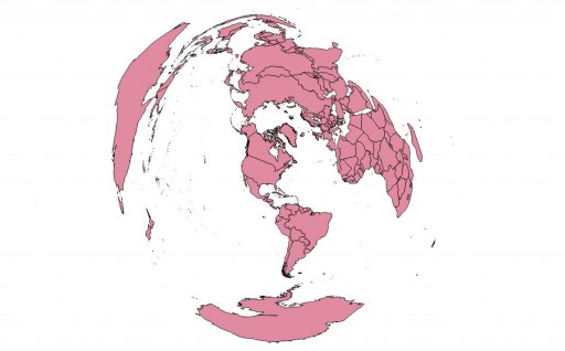
The lat_0 and lon_0 parameters are just where you want the centre of the map to be. Things get a bit odd if you try to plot the whole world:

The antipodes get plotted underneath, and everything looks messed up. I may have to take my question to GIS – Stack Exchange to see if I can find an answer. Still, for all its wrongness, you can make something pretty, like my whole world Maidenhead locator grid projected this way turns into a rose:

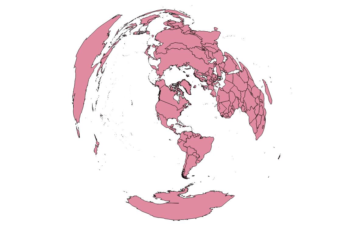
Update: André advised on Stack Exchange that you need to specify the correct radius:

ogr2ogr -t_srs "+proj=aeqd  +lat_0=43.7308 +lon_0=-79.2647 +R=6371000" va3pid-world.shp TM_WORLD_BORDERS_SIMPL-0.3.shp

This works rather well:

aeqd-qgis


Categories
GIS

binning by angle

I was trying to sort a series of polar coordinates by compass direction: everything in the N sector, then NNE, NE, ENE, E, … This is trickier than it looks, since the North sector includes angles between 348.75° and 11.25°.

It’s easier to think of the problem instead of being one of N bins centred on 0°, but rather one of 2N bins starting at 0°. Then, all one needs to do is shift everything round by one of these half bins (so +1, modulo 2N), then divide the number of bins back to the number we want. Done!

Here’s some code to do it. It may look like C-like pseudocode, but it’s real live AWK:

function bin(angle,nbins){
  return int(((int(angle/(360.0/(nbins*2)))+1)%(nbins*2))/2);
}

You probably want the angles to be between 0..360°. But you knew that.

Categories
GIS

Drawing Eggs

When designing wind farms, you need to keep the turbines a certain distance apart from one another. If you don’t, the wakes from the turbines reduce efficiency, and the turbulence can reduce the warranted life of the machine. Typically, a manufacturer might specify a minimum downwind separation of 5 diameters, and a crosswind separation of 3 diameters. It’s an easy check with a buffer overlap, but these buffers are elliptical, which not all GIS packages can draw.

Take, for example, the following three points designated as (completely made-up)  wind turbine locations:

name    XCOORD           YCOORD
1    557186.675000    4757125.590000
2    557447.931000    4756968.690000
3    557664.999000    4756817.810000

These look quite far apart, even if you were using large, 100+m diameter wind turbines:

But if we have a wind direction of 210°, downwind/crosswind separation of 5D & 3D respectively, and a 101m diameter rotor, it’s not so good:

Turbines 2 & 3 are too close together; the ellipses shouldn’t touch.

As awk is the only scripting language I have on my work computer, I wrote the script that generates the buffer shapefile in awk. The script calls Frank’s Shapefile C Library utilities to actually make the shapefile. Here’s the code:

#!/bin/awk -f
# draw an ellipse based on turbine location to generate
#  for WTG separation buffer
# scruss - 2011-09-27

# assumes that stdin has three columns:
#  1 - label
#  2 - x coordinate
#  3 - y coordinate

# variables:
#  diameter = rotor diameter
#  cross = crosswind separation, diameters
#  down = downwind separation, diameters
#  wind = prevailing wind direction
#  base = base for shape file name

BEGIN {
	OFMT="%.1f";
	CONVFMT="%.1f";
	OFS=" ";

	if (diameter < 0) {
		print "diameter must be set";
		exit;
	}

	if (cross < 0) {
		print "cross must be set";
		exit;
	}

	if (down < 0) {
		print "down must be set";
		exit;
	}

	if (down < cross) {
		print "down must be greater than cross";
		exit;
	}

	if (wind < 0) {
		print "wind must be set";
		exit;
	}

	if (base ~ /^$/) {
		print "base must be a string";
		exit;
	}

	pi = 3.141592654; # I know, I know ...
	# calc cartesian angle from wind bearing, in radians
	beta = ((450 - wind)%360) * pi/180;

	# output shapelib tools init commands
	print "dbfcreate " base " -s name 40";
	print "shpcreate " base " polygon";
}

# for every line
{
	name=$1;
	x=$2;
	y=$3;

	major = diameter * down/2;
	minor = diameter * cross/2;
	first="";
	points="";
	maxn=36;
	for (i=0; i<maxn; i++) {
	    alpha = (i * (360/maxn)) * pi/180;
	    x1 = x + major * cos(alpha) * cos(beta) - minor * sin(alpha) * sin(beta);
	    y1 = y +  major * cos(alpha) * sin(beta) + minor * sin(alpha) * cos(beta);
	    if (i == 0) { # store the first point
		first= x1 " " y1;
	    }
	    points = points  " " x1 " " y1;
	}
	points = points  " " first;
	print "dbfadd " base ".dbf " name;
	print "shpadd " base, points;
}

awk is charmingly odd in that you can specify variable on the command line. Here’s how I called it, with the above coordinates as input:

awk -v diameter=101 -v cross=3 -v down=5 -v wind=210 -v base="fakewtg-ellipse" -f separation.awk

Pipe the output through a shell, and there are your ellipses.