@MaptimeTO asked me to summarize the brief talk I gave last week at Maptime Toronto on making maps from the Technical and Administrative Frequency List (TAFL) radio database. It was mostly taken from posts on this blog, but here goes:
One of the many constraints in building wind farms is allowing for radio links. Both the radio and the wind industries have agreed on a process of buffering and consultation. Here’s how I handled it in Python: Making weird composite shapes with Shapely.
The format is a real delight for all legacy-data nerds: aka a horrible mess of conditional field widths and arcane numeric codes. I wrote a SpatiaLite SQL script to make sense of it all: scruss/taflmunge. This (kind of) explains what it does: TAFL — as a proper geodatabase.
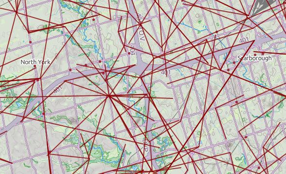
Here’s a raw dump (very little metadata, sorry) from 2013 in the wonderful uMap: Ontario Microwave Links.
In a fabulous piece of #opendatafail, Industry Canada have migrated all the microwave data (so, all links ≥ 960 MHz) to a new system which doesn’t work yet, and also stripped out all of the microwave data from recent TAFL files. They claim to be fixing it, but don’t hold your breath. If you want data to play with, here’s Ontario’s data from October 2013 (nb: huge) — ltaf_ont_tafl-20131001.
Update, 2017: TAFL now seems to be completely dead, and Spectrum Management System has replaced it. None of the records appear to be open data, and the search environment seems — if this is actually possible — slower and less feature-filled than in 2013.
Update, 2013-08-13: Looks like most of the summary pages for these data sets have been pulled from data.gc.ca; they’re 404ing. The data, current at the beginning of this month, can still be found at these URLs:
I build wind farms. You knew that, right? One of the things you have to take into account in planning a wind farm is existing radio infrastructure: cell towers, microwave links, the (now-increasingly-rare) terrestrial television reception.
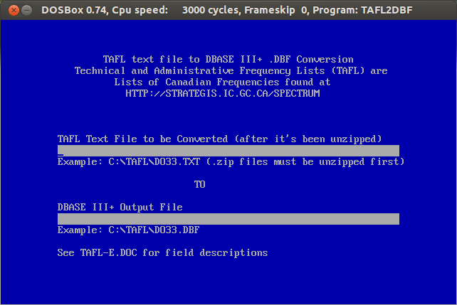
Wrestle with the Spectrum Direct website, which can’t handle the large search radii needed for comprehensive wind farm design. At best, it spits out weird fixed-width text data, which takes some effort to parse.
Download the Technical and Administrative Frequency Lists (TAFL; see update above for URLs), and try to parse those (layout, fields). Unless you’re really patient, or have mad OpenRefine skillz, this is going to be unrewarding, as the files occasionally drop format bombs like
Yes, you just saw conditional different fixed-width fields in a fixed-width text file. In my best Malcolm Tucker (caution, swearies) voice I exhort you to never do this.
So searching for links is far from obvious, and it’s not like wireless operators do anything conventional like register their links on the title of the properties they cross … so these databases are it, and we must work with them.
That’s why I wrote taflmunge. It currently does one thing properly, and another kinda-sorta:
For all TAFL records fed to it, generates a SpatiaLite database containing these points and all their data; certainly all the fields that the old EXE produced. This process seems to work for all the data I’ve fed to it.
Tries to calculate point-to-point links for microwave communications. This it does less well, but I can see where the SQL is going wrong, and will fix it soon.
taflmunge runs anywhere SpatiaLite does. I’ve tested it on Linux and Windows 7. It’s just a SQL script, so no additional glue language required. The database can be queried on anything that supports SQLite, but for real spatial cleverness, needs SpatiaLite loaded. Full instructions are in the taflmunge / README.md.
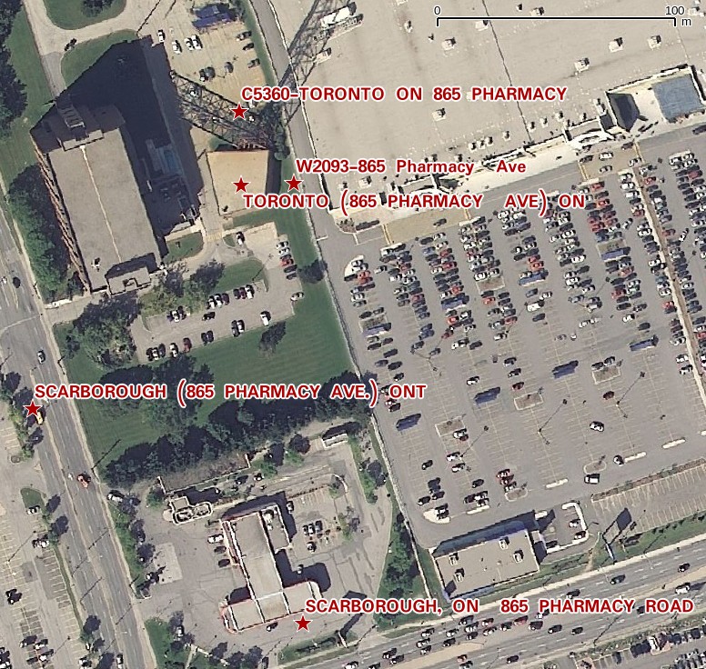
TAFL is clearly maintained by licensees, as the data can be a bit “vernacular”. Take, for example, a tower near me:
The tower is near the top of the image, but the database entries are spread out by several hundred meters. It’s the best we’ve got to work with.
Ultimately, I’d like to keep this maintained (the Open Data TAFL files are updated monthly), and host it in a nice WebGIS that would allow querying by location, frequency, call sign, operator, … But that’s for later. For now, I’ll stick with refining it locally, and I hope that someone will find it useful.
Something I used to have to do a lot was to maintain a table of the nearest houses to prospective wind farm layouts. While the list of houses didn’t change very much, the layouts did. I came up with an only semi-unwieldy spreadsheet to do the calculations. The table was ultimately used in submissions to the Ontario Ministry of the Environment.
I’ve mapped out a trivially small example below; three houses, three wind turbines. In real life, there would be hundreds of each.
Sorry to include it as an image, but WordPress really doesn’t like pasted tables. If you really must, the text content is below the fold.
Though it’s small, it’s a bit of a horror, so you might want to download near.ods (opendocument spreadsheet). The mauve section contains the house coordinates, the blue the turbines. The green section is a simple Cartesian distance calculator (√(Δx2+Δy2)) for those coordinates. The beige (or orange; or is it salmon?) bit is where things get difficult. Finding the closest distance is easy with the MIN function. Finding the column heading in which that minimum distance occurs is a bit more tricky, using INDIRECT, ADDRESS, COLUMN and MATCH to pull out the contents of the cell. This is one of the few spreadsheets I’ve written that will break if you rearrange it; hardcoded cell address mathematics will do that.
Getting the same result in SQL is little more difficult. I mean, I can make the table of distances easily enough:
select houses.ref as House,
 turbines.id as Turbine,
 distance(houses.geom, turbines.geom) as Distance
from houses, turbines
order by House, Turbine
but producing a nice compact table of houses, the nearest turbine, and the distance will need more pondering.
In my first post I asked where am i? The gps in my phone said I was standing at 43.73066°N, 79.26482°W. In real life, I was standing at the junction of Kenmark Blvd and Chevron Cres.
With the Open Toronto centreline data, I can check the location of road intersections:
select distinct (
astext (
transform (
intersection ( r1.geometry, r2.geometry ), 4326
 ) ) )
from centreline as r1, centreline as r2
where r1.lf_name = 'KENMARK BLVD' and r2.lf_name
 = 'CHEVRON CRES'
Hmm; three answers. NULL I can’t answer; I’ll put it down as an exhortation to Be Here Now. The second is given a clue by one of the street names: Chevron Crescent – first thing I learned when I had my newspaper round is that a crescent’s going to end you up back on the same road you started from. The last one, though, agrees to 5(ish) decimal places – well within the accuracy of my simple GPS.
Update: This query gets really, really slow on long streets. Both Chevron and Kenmark only have two road segments. Kennedy and Steeles East each have over 90.
If you consider Toronto to be defined by its city wards, the centre of Toronto lies at 43.725518°N, 79.390531°W.
If you consider Toronto to be defined by its neighbourhoods, the centre of Toronto lies at 43.726495°N, 79.390641°W.
You can work this out in one line of SQL. By combining all the wards or neighbourhoods into one union shape (SpatiaLite uses the GUnion() function), and then calculating the centroid, that’s the centre of the city:
select astext(transform(centroid(gunion(geometry)),4326)) from wards
To get the results in a more human-friendly format, I transformed it to WGS84 (EPSG SRID 4326), and used astext() to get it in something other than binary.
Well, almost. The DBF component of a shapefile seems somewhat resistant to adding a column, and SQLite doesn’t seem very happy with its ALTER TABLE ADD COLUMN ... syntax.
As usual, I needed to create the database table from the shapefile. I’m not bothered about CRS, so I used -1.
I had mixed success getting data to load into this new column. So I improvised.
!!! WARNING: EGREGIOUS MISUSE OF DATA FOLLOWS !!!
(Sensitive readers are advised to look away)
There’s a seeming unused numeric column SHAPE_LEN in the table. As my new candidates column was coming up with occasional nulls, I cheated:
UPDATE Wards set shape_len=3 where scode_name="1"

UPDATE Wards set shape_len=1 where scode_name="2"

UPDATE Wards set shape_len=0 where scode_name="3"

...

UPDATE Wards set shape_len=3 where scode_name="44";
I then added SHAPE_LEN as the label, and defined a range based colour gradient for the wards in QGIS’s layer properties:
And this is how it looks:
Another partial success, as Professor Piehead would say.
My post diary of a geonumpty to my main blog is really what got me started thinking about abstract geographic data. In it, I (with a lot of external help) develop queries to count points in areas with the same owner, and find points outside properties.
I’m going to use SpatiaLite and the Toronto One Address Repository to try some simple geocoding. That is, given an address, spit out the real-world map coordinates. As it happens, the way the Toronto data is structured it doesn’t really need to use any GIS functions, just some SQL queries. There are faster and better ways to code this, but I’m just showing you how to load up data and run simple queries.
SpatiaLite is my definition of magic. It’s an extension to the lovely SQLite database that allows you to work with spatial data – instead of selecting data within tables, you can select within polygons, or intersections with lines, or within a distance of a point.
I’m going to try to avoid having too many maps here, as maps are a snapshot of a particular view of a GIS at a certain time. Maps I can make; GIS is what I’m trying to learn.
So, download the data and load up SpatiaLite GUI. Here I’ve created a new database file. addresses.sqlite. I’m all ready to load the shapefile.
Shapefiles are messy things, and are definitely glaikit. Firstly, they’re a misnomer; a shapefile is really a bunch of files which need to be kept together. They’re also a really old format; the main information store is actually a dBaseIII database. They also have rather dodgy ways of handling projection metadata. For all their shortcomings, no-one’s come up with anything better that people actually use.
Projection information is important, because the world is inconveniently unflat. If you think of a projected X-Y coordinate system as a graph paper Post-It note stuck to a globe, the grid squares depend on where you’ve decided to stick the note. Also, really only the tiny flat part that’s sticking to the globe closely approximates to real-world coordinates.
Thankfully, the EPSG had a handle on all this projection information (and, likely, Post-It notes). Rather than using proprietary metadata files, they have a catalogue of numbers that exactly identify map projections. SpatiaLite uses these Spatial Reference System Identifiers (SRIDs) to keep different projections lined up.
Toronto says its address data is in ‘MTM 3 Degree Zone 10, NAD27’. That’s not a SRID. You can list all the SRIDs that SpatiaLite knows with:
select * from spatial_ref_sys
which returns over 3500 results.
As we know there’s an MTM (Modified Transverse Mercator) and a 27 in the title, we can narrow things down:
select srid,ref_sys_name from spatial_ref_sys where ref_sys_name like '%MTM%' and ref_sys_name like '%27%'
The results are a bit more manageable:
srid
ref_sys_name
2017
NAD27(76) / MTM zone 8
2018
NAD27(76) / MTM zone 9
2019
NAD27(76) / MTM zone 10
2020
NAD27(76) / MTM zone 11
2021
NAD27(76) / MTM zone 12
2022
NAD27(76) / MTM zone 13
2023
NAD27(76) / MTM zone 14
2024
NAD27(76) / MTM zone 15
2025
NAD27(76) / MTM zone 16
2026
NAD27(76) / MTM zone 17
32081
NAD27 / MTM zone 1
32082
NAD27 / MTM zone 2
32083
NAD27 / MTM zone 3
32084
NAD27 / MTM zone 4
32085
NAD27 / MTM zone 5
32086
NAD27 / MTM zone 6
So it looks like 2019 is our SRID. That last link goes to spatialreference.org, who maintain a handy guide to projections and SRIDs. (Incidentally, Open Toronto seems to use two different projections for its data – the other is ‘UTM 6 Degree Zone 17N NAD27’ with a SRID of 26717.)
So let’s load it:
This might take a while, as there are over 500,000 points in this data set.
If you want to use this data along with more complex geographic queries, add a Spatial Index by right-clicking on the Geometry table and ‘Build Spatial Index’. This will take a while again, and make the database file quite huge (128MB on my machine).
Update: there’s a much quicker way of doing this without messing with invproj in this comment.
Now we’re ready to geocode. I was at the Toronto Reference Library today, which is at 789 Yonge Street. Let’s find that location:
select easting, northing, address, lf_name, name, fcode_desc from TCL3_ADDRESS_POINT where lf_name like 'yonge%' and address=789
which gives:
EASTING
NORTHING
ADDRESS
LF_NAME
NAME
FCODE_DESC
313923.031
4836665.602
789
YONGE ST
Toronto Reference
Library
(for most places, NAME and FCODE_DESC are blank.)
Ooooh … but those coordinates don’t look anything like the degrees we had yesterday. We have to convert back to unprojected decimal degrees with my old friend, proj. If we store the northing, easting and a label in a file, we can get the get the geographic coordinates with:
Now that’s more like it: 43.671824°N, 79.386869°W. On a map, that’s:
Pretty close, eh?
Incidentally, I didn’t just magic up that weird invproj line. Most spatial databases use proj to convert between projections, and carry an extra column with the command line parameters. For our SRID of 2019, we can call it up with this:
select proj4text from spatial_ref_sys where srid=2019;
 @MaptimeTO asked me to summarize the brief talk I gave last week at Maptime Toronto on making maps from the Technical and Administrative Frequency List (TAFL) radio database. It was mostly taken from posts on this blog, but here goes:
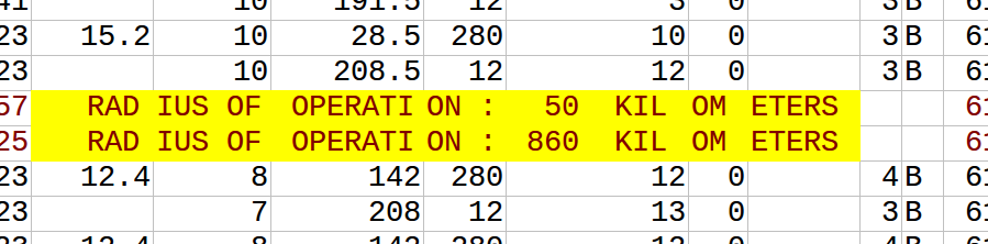


 This might take a while, as there are over 500,000 points in this data set.