Categories
GIS

Some notes on the wartime “Modified British” map coordinate systems

Growing up in a small country, I assumed the whole world used metric grid map coordinates. I mean, why would anyone bother with those tedious latitudes and longitudes when you could have your location defined by something as neat as NS539555?

The tidy, militaristic Ordnance Survey came up with the National Grid reference system, where large grid squares were given letters, and the rest of the reference was given numerically. Wikipedia gives a better graphical explanation than I could:

Illustration of the Ordnance Survey National Grid coordinate system, with Trafalgar Square as an example [CC BY-SA 3.0]

During WW2, the UK war office extended this system across most of Europe. Since most European countries didn’t use exactly the same Transverse Mercator projection as the UK did, a number of existing mapping systems were pressed into use, but using the same interleaved alphanumeric format as the OS grid reference.

The reference site for these systems is Thierry Arsicaud’s excellent Notes on the “Modified British System” used on the European Theatre of Operations during the WWII. Thierry, however, wasn’t trying to use these historical map references in a GIS, so his work needs a little massage to get to be used with QGIS.

In this example, I’m going to concentrate on the South Italy zone, as that’s where I was asked to look at some war diaries from 1943. The system is similar to the OS grid, but the main difference is that the major grid reference is often given in lower case. So RN in OSGB would most often be denoted rN in the Modified British system. Both would refer to a 100 km square at (700, 700) km from the origin. (The exceedingly nitpicky might point out that RN is never used in the UK as it’s somewhere in the Atlantic, west of Ireland. To them, I say: Well, bless your heart)

The key to both the OSGB grid and the Modified British system is a 2500 × 2500 km square, split into 25 500 km squares, and given a letter, az with i excluded:

mod_brit-major

Each letter encodes both an easting and a northing; so r is (500000, 500000). About the easiest way to unpack this encoding is through a simple string lookup:

result = SEARCH(letter, "VWXYZQRSTULMNOPFGHJKABCDE")-1
easting = result MOD 5
northing = INT(result / 5)

where SEARCH is a function which returns the position of a letter in a string (so SEARCH(“V”, “VWXYZ…”) returns 1).

When applied as per the GSGS South Italy system, you get something like this:

italy_south-major-r

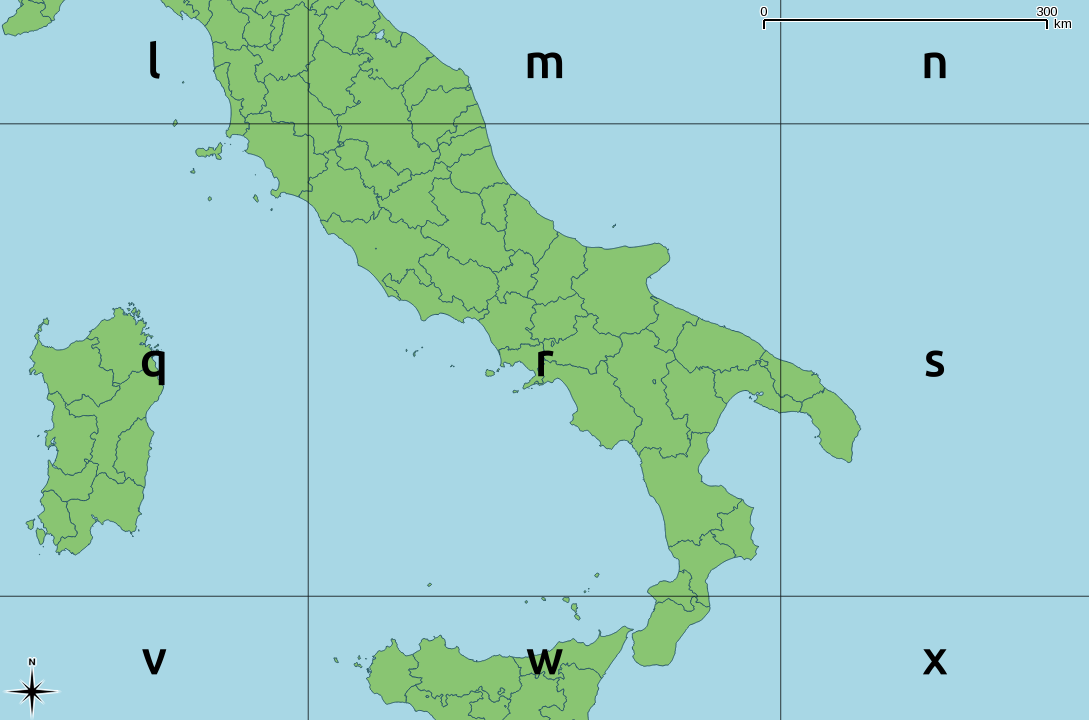
These major grid squares are in turn split into 25 minor squares of 100 km side:

mod_brit-minor

Or overlaid on a map:

italy_south-minor-r

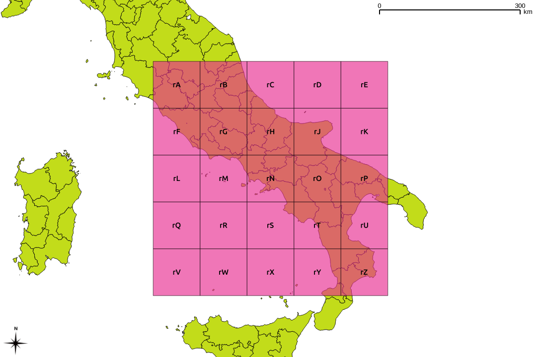
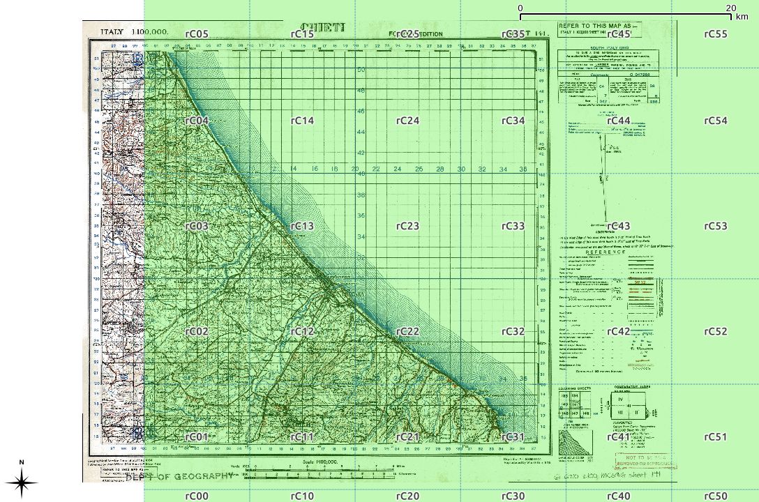
For grid references of higher precision, a series of numbers is appended. There should always be an even count of these numbers, for reasons which should become clear soon. Here is the rC square, split into 10 km references:

mod_brit-rC

These two digit references are about the shortest/least precise you might ever see. Overlaid on an appropriate sheet from the McMaster archive WWII Topographic Map Series (which are CC BY-NC; for which, many thanks), you get:

chieti-rC_grid

The actual projection details are given on each map:

south_italy

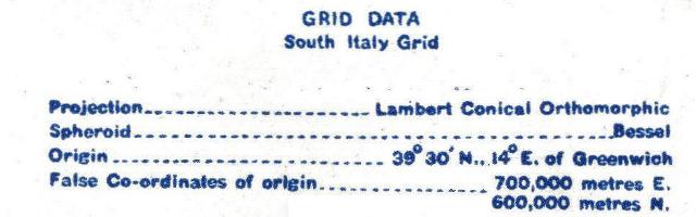
We can turn this into a PROJ.4 definition:

Projection - Lambert Conical Orthomorphic  →    +proj=lcc
Ellipsoid: Bessel 1841                     →    +ellps=bessel
False Easting : 700000                     →    +x_0=700000
False Northing : 600000                    →    +y_0=600000
Central Meridian : 14.0°                   →    +lon_0=14 
Central Parallel : 39.5°                   →    +lat_0=39.5 +lat_1=39.5
Scale Factor : 0.99906                     →    +k_0=0.99906
                       (other proj.4 terms)     +units=m +no_defs  

or in one line,

+proj=lcc +lat_0=39.5 +lat_1=39.5 +lon_0=14 +k_0=0.99906 +x_0=700000 +y_0=600000 +ellps=bessel +units=m +no_defs

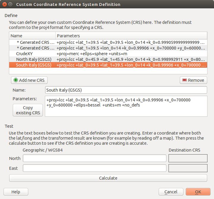
In QGIS, you can plug those values into the Custom CRS manager, and you will be able to work in these antiquated coordinate systems with ease:

Screenshot from 2015-01-09 07:28:53

I haven’t yet quite managed to work out some of the other GSGS coordinate systems. My work on North Italy is a stubborn 100 km off true, for no well-defined reason. I haven’t managed to work out unpicking alphanumeric grid references into geometries automatically, either. These will come later.

Finally, some of the coordinates you might see might not meet these specifications. In the limited survey I’ve done, I’ve noted:

  1. references with the major grid missing, so rCxy… was written as Cxy….
  2. references to ‘MR’ (map reference), with no alphanumeric part, such as MR 322142 (from here), which would be more correctly given as rC322142.

Huge thanks to Thierry Arsicaud, both for the great reference website, and also for the e-mail correspondence helping explain the parameters for the GSGS Italy South system. Props too to the Geographic Information Systems Stack Exchange folks for help with working out the proj.4 settings.

Categories
GIS

Not really getting the Azimuthal Equidistant projection right

Update: thanks to André, this works! See the updated ogr2ogr line.

All I really wanted to do is make a map like this:

This is an Azimuthal Equidistant projection, with me at the centre (of course) and the rest of the world spread out in a fan by distance and bearing. It’s somewhat surprising to find that South Africa is almost directly east of Toronto, and New Zealand to the southwest.

If I had a directional antenna and a rotor, this map would show me where I would have to point the antenna to contact that part of the world. I can’t rotate my dipole (unless I commit some unauthorized local plate tectonics) so I’m stuck with where my antenna transmits and receives best.

The above map was made with AZ_PROJ, a PostScript program of some complexity for plotting world maps for radio use. The instructions for installing and running AZ_PROJ are complex and slightly dated. I got the above output running it through Ghostscript like this:

gs -sDEVICE=pdfwrite -sOutputFile=va3pid_world.pdf az_ini.ps -- az_proj.ps world.wdb

The format of the az_ini.ps file is complex, and I’m glad I’m an old PS hacker to be able to make head or tail of it.

For all its user-hostility, AZ_PROJ is powerful. Here’s a version of the map I wanted all along:

This shows my furthest QSO in each of the 16 compass directions. (You might note that North is empty: my furthest contact in that direction is some 13km away, whether by lack of folks in that sector or dodginess of my antenna.) Contrast that with my Mercator QSO map, and you’ll see that Azimuthal Equidistant is a much better projection for this application.

To show how radically different the world looks to different people, here’s the world according to my mate Rob in Hamilton, NZ:

I’d been trying to use OGR to transform arbitrary shapefiles into this projection. For maps entirely contained within the same hemisphere (so having extent less than ±90° in any cardinal direction), this works:

ogr2ogr -t_srs "+proj=aeqd  +lat_0=43.7308 +lon_0=-79.2647" out.shp in.shp

The lat_0 and lon_0 parameters are just where you want the centre of the map to be. Things get a bit odd if you try to plot the whole world:

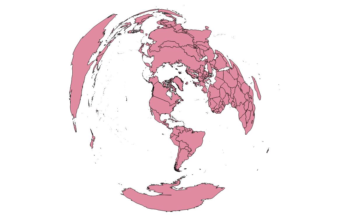
The antipodes get plotted underneath, and everything looks messed up. I may have to take my question to GIS – Stack Exchange to see if I can find an answer. Still, for all its wrongness, you can make something pretty, like my whole world Maidenhead locator grid projected this way turns into a rose:

Update: André advised on Stack Exchange that you need to specify the correct radius:

ogr2ogr -t_srs "+proj=aeqd  +lat_0=43.7308 +lon_0=-79.2647 +R=6371000" va3pid-world.shp TM_WORLD_BORDERS_SIMPL-0.3.shp

This works rather well:

aeqd-qgis


Categories
GIS

proj.4 init annoyances: it’s all apple’s fault

I was going to write a rant about how Ubuntu sets up proj.4 init files incorrectly, then I found that the problem actually lies with OS X. OS X is unusual for a Unix variant, as it uses a case-insensitive file system; flarp.txt is the same as FLARP.TXT. Under more traditional Unices, they’d be different files.

Most of the examples on this blog were written under OS X, and I was concerned when they didn’t work under Ubuntu. It seems that proj.4 uses a very simple way of defining initialization files. If you specify, say, “+init=EPSG:2958”, proj digs around in its configuration files for a file called EPSG, then searches for an identifier in that file which matches the ID 2958. Under OS X, you can specify EPSG, epsg, or even EpSg – they all work. Under Ubuntu, using anything other that epsg fails with this message:

<proj>:
projection initialization failure
cause: no system list, errno: 2

In short, use lower case init specifications, and it’ll work everywhere.

It seems that there are some other applications (mapserver?) that have problems calling proj, so if you’re seeing this error and it’s not something you can correct from the command line:

  1. Find out where your installation keeps its initialization files. You can do this by setting PROJ_DEBUG=1:
    PROJ_DEBUG=1 proj +init=epsg:2958
    and you should get a message like:
    pj_open_lib(epsg): call fopen(/usr/share/proj/epsg) - succeeded
  2. cd /usr/share/proj (or wherever the last command said the epsg file was located)
  3. sudo ln -s epsg EPSG

Now your installation should work no matter which case you use. Camel case, unfortunately, excluded.

Categories
GIS

three norths to choose from

North is a slippery thing, a trickster. There are at least three norths to choose from:

  • Magnetic north – where the compass needle points. Currently way in the northwest of Canada, it’s scooting rapidly towards Siberia. Come baaack, magnetic north! Was it something we said?
  • True north – straight up and down on the axis of this planet.
  • Grid north – the vertical lines on your map. Due to the earth’s curvature, there’s only one line on a grid that exactly coincides with true north. Away from that line, there’s a correction that you need to apply.

That grid to true correction is what I’m looking at today. In my work, I need to work out where shadows of wind turbines fall. I work in grid coordinates, so I need to correct for true north sun angles. Here’s a shell script that uses familiar programs invproj and geod to work out the local true north correction:

#!/bin/sh
# gridnorth.sh - show the grid shift angle at a certain point
# created by scruss on Sun 4 Apr 2010 18:19:29 EDT
# $Id: gridnorth.sh,v 1.2 2010/04/05 12:23:57 scruss Exp $

# you might want to change this
srid=2958

# two arguments mandatory, third optional
if
 [ $# -lt 2 ]
then
 echo Usage: $0 x y [srid]
fi

# truncate arguments to integers so the shell maths will work
x=`echo $1 | sed 's/\.[0-9]*//;'`
y=`echo $2 | sed 's/\.[0-9]*//;'`
# calculate points 1000 units (grid) south and north of the chosen point
lowy=$((y-1000))
highy=$((y+1000))

if
 [ $# -eq 3 ]
then
 srid=$3
fi

min=`echo $lowy  $x foo | invproj -r -f &amp;amp;quot;%.6f&amp;amp;quot; +init=EPSG:$srid`
max=`echo $highy $x foo | invproj -r -f &amp;amp;quot;%.6f&amp;amp;quot; +init=EPSG:$srid`
minlon=`echo $min | awk '{print $1;}'`
minlat=`echo $min | awk '{print $2;}'`
maxlon=`echo $max | awk '{print $1;}'`
maxlat=`echo $max | awk '{print $2;}'`
echo $minlat $minlon $maxlat $maxlon |\
 geod +ellps=WGS84 -f &amp;amp;quot;%.3f&amp;amp;quot; -p -I +units=m |\
 awk '{print $1;}'

The script is called with two arguments (the easting and the northing) and an optional third argument, the SRID for the current projection:

$ ./gridnorth.sh 639491 4843599 26717
1.198

The value returned is the angle (clockwise) that grid north differs from true north. Unless you’re using the same SRID that I’ve put in the script as default, you probably want to specify (or change) it.

So how do I know if this is even remotely correct? If you look at any CanMatrix scanned topographic map (either Print Ready or Georeferenced). there’s a declination indicator shown:

That’s the map eastern Toronto is in; its sheet reference is 030M11. We’ll ignore the magnetic declination for now, as 1984 is way out of date, and there is much to be said on geomagnetism that I don’t understand.  The map says its centre is 1° 12′ clockwise of true north. The centre of the map is approximately 641500E, 4831000N (UTM Zone 17N NAD27; EPSG 26717; or in real terms, in the lake, a few klicks SE of Ashbridges Bay) so:

$ ./gridnorth.sh 641500 4831000 26717
1.209

1° 12′ is 1.2, so I think I’m officially pretty durn close.

To show that grid skew changes across the map, the upper right hand corner of the map is 660000E, 4845000N, which is off by 1.375°.

Categories
Uncategorized

current tools of my trade

Mark asked: What kind of GIS software are you using?
Well, since you asked:-

  • SpatiaLite: spatial awesome built on SQLite. I love it because I don’t need to play DBA.
  • QGIS: for maps
  • ogr: for file format futzing
  • proj: for scrupulously correct (well, if I knew what I was doing …) conversion between projected and otherwise.
  • OpenOffice: for those tedious calculations
  • … and about 20 years of unix experience to mash all the results together.

All of the above are free. I’m doing this because I want to learn. Asking elsewhere hasn’t turned up anything useful.

Categories
GIS

a simple geocoder for toronto

I’m going to use SpatiaLite and the Toronto One Address Repository to try some simple geocoding. That is, given an address, spit out the real-world map coordinates. As it happens, the way the Toronto data is structured it doesn’t really need to use any GIS functions, just some SQL queries. There are faster and better ways to code this, but I’m just showing you how to load up data and run simple queries.

SpatiaLite is my definition of magic. It’s an extension to the lovely SQLite database that allows you to work with spatial data – instead of selecting data within tables, you can select within polygons, or intersections with lines, or within a distance of a point.

I’m going to try to avoid having too many maps here, as maps are a snapshot of a particular view of a GIS at a certain time. Maps I can make; GIS is what I’m trying to learn.

So, download the data and load up SpatiaLite GUI. Here I’ve created a new database file. addresses.sqlite. I’m all ready to load the shapefile.

Shapefiles are messy things, and are definitely glaikit. Firstly, they’re a misnomer; a shapefile is really a bunch of files which need to be kept together. They’re also a really old format; the main information store is actually a dBaseIII database. They also have rather dodgy ways of handling projection metadata. For all their shortcomings, no-one’s come up with anything better that people actually use.

Projection information is important, because the world is inconveniently unflat. If you think of a projected X-Y coordinate system as a graph paper Post-It note stuck to a globe, the grid squares depend on where you’ve decided to stick the note. Also, really only the tiny flat part that’s sticking to the globe closely approximates to real-world coordinates.

Thankfully, the EPSG had a handle on all this projection information (and, likely, Post-It notes). Rather than using proprietary metadata files, they have a catalogue of numbers that exactly identify map projections. SpatiaLite uses these Spatial Reference System Identifiers (SRIDs) to keep different projections lined up.

Toronto says its address data is in ‘MTM 3 Degree Zone 10, NAD27’. That’s not a SRID. You can list all the SRIDs that SpatiaLite knows with:

select * from spatial_ref_sys

which returns over 3500 results.

As we know there’s an MTM (Modified Transverse Mercator) and a 27 in the title, we can narrow things down:

select srid,ref_sys_name from spatial_ref_sys where ref_sys_name like '%MTM%' and ref_sys_name like '%27%'

The results are a bit more manageable:

srid ref_sys_name
2017 NAD27(76) / MTM zone 8
2018 NAD27(76) / MTM zone 9
2019 NAD27(76) / MTM zone 10
2020 NAD27(76) / MTM zone 11
2021 NAD27(76) / MTM zone 12
2022 NAD27(76) / MTM zone 13
2023 NAD27(76) / MTM zone 14
2024 NAD27(76) / MTM zone 15
2025 NAD27(76) / MTM zone 16
2026 NAD27(76) / MTM zone 17
32081 NAD27 / MTM zone 1
32082 NAD27 / MTM zone 2
32083 NAD27 / MTM zone 3
32084 NAD27 / MTM zone 4
32085 NAD27 / MTM zone 5
32086 NAD27 / MTM zone 6

So it looks like 2019 is our SRID. That last link goes to spatialreference.org, who maintain a handy guide to projections and SRIDs. (Incidentally, Open Toronto seems to use two different projections for its data – the other is ‘UTM 6 Degree Zone 17N NAD27’ with a SRID of 26717.)

So let’s load it:

This might take a while, as there are over 500,000 points in this data set.

If you want to use this data along with more complex geographic queries, add a Spatial Index by right-clicking on the Geometry table and ‘Build Spatial Index’. This will take a while again, and make the database file quite huge (128MB on my machine).

Update: there’s a much quicker way of doing this without messing with invproj in this comment.

Now we’re ready to geocode. I was at the Toronto Reference Library today, which is at 789 Yonge Street. Let’s find that location:

select easting, northing, address, lf_name, name, fcode_desc from TCL3_ADDRESS_POINT where lf_name like 'yonge%' and address=789

which gives:

EASTING NORTHING ADDRESS LF_NAME NAME FCODE_DESC
313923.031 4836665.602 789 YONGE ST Toronto Reference Library

(for most places, NAME and FCODE_DESC are blank.)

Ooooh … but those coordinates don’t look anything like the degrees we had yesterday. We have to convert back to unprojected decimal degrees with my old friend, proj. If we store the northing, easting and a label in a file, we can get the get the geographic coordinates with:

invproj -E -r -f "%.6f" +proj=tmerc +lat_0=0 +lon_0=-79.5 +k=0.9999 +x_0=304800 +y_0=0 +ellps=clrk66 +units=m +no_defs < file.txt

which gives us:

4836665.602000	313923.031000	-79.386869	43.671824	Library

Now that’s more like it:  43.671824°N, 79.386869°W. On a map, that’s:

Pretty close, eh?

Incidentally, I didn’t just magic up that weird invproj line. Most spatial databases use proj to convert between projections, and carry an extra column with the command line parameters. For our SRID of 2019, we can call it up with this:

select proj4text from spatial_ref_sys where srid=2019;

which returns:

+proj=tmerc +lat_0=0 +lon_0=-79.5 +k=0.9999 +x_0=304800 +y_0=0 +ellps=clrk66 +units=m +no_defs

Update: there’s a much better way of invoking invproj. It understands EPSG SRIDs, so we could have done:

invproj -E -r -f "%.6f" +init=EPSG:2019 < file.txt