Categories
GIS

toronto’s human centre

Since it was trivial to calculate the centre of the city, I thought I’d do something a little more complex: calculate the centre of the city, weighted for population. I scraped the 2006 population data by ward from the City of Toronto: Ward Profiles pages; hooray for curl and regexes. Realising that I had no information on population distribution within wards, I made a good old engineering assumption: we could idealize the population as a point mass at the centroid of each ward, and then calculate the centre of mass by balancing moments around the X and Y axis. (I mean, c’mon – it’s the sort of thing we all think about daily … isn’t it? Guys … hello … anyone there?)

I’ll spare you the details until after the jump, but I calculate the human centre of Toronto to be at 43.717794°N, 79.390299°W – that’s in Blythwood Ravine, just south of Blythwood Road. We should have a picnic there …

Categories
Uncategorized

Japanese Map Symbol for a windmill

I’m rather taken with the symbol that Japanese maps use for wind mills and wind turbines. I’ll try to modify it for use in QGis.

Update: so how does this look?

I cleaned up the blade angles, added line end-caps, and made all the white bits transparent. Works fine in QGis.

Categories
GIS

a minor revelation about road segments

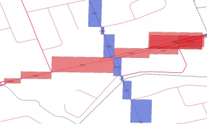
I’m still learning how Toronto encodes its roads – and whether this is a common practice. Between intersections, roads are stored as polyline segments. Kennedy Road (blue) and Eglinton Ave E (red) are shown below as a series of road segment minimum bounding rectangles (MBR):


I was hoping it would be quick and easy to find the MBR of the whole street, then search for intersections only in the intersections of the MBRs. On an orthogonal grid (even a squinty one) this would save a bunch of searching.

I don’t know if I can use the fact that the end points of road sections are common at intersections. I really am a geonumpty.

All this may soon be moot, as I hear that the next release of the toronto.ca | Open data – expected early April – will have explicit intersection data. Yay!

Categories
GIS

Toronto’s Angles

As many Canadians will tell you, most Torontonians are a bit skewed. While others might have different explanations, I put it down to our road grid. What we call north in the city is actually some 16.7° west of north.

While we do have a perpendicular grid, it’s twisted to the left (steady, Edmontonians). I attempted to work out what the average angle is.

I eyeballed several long straight streets, and picked out representative intersections. Finidng the coordinates of these intersections took a surprisingly long time, as each street has several road sections. To find an intersection, each section on one road has to be queried against each section of the other. It gets there, eventually.

To save the tedium of showing the queries, here are the results. The angles are anticlockwise from the X-axis.

N-S	 Intersection1 Intersection2 Angle
======== ============= ============= ======
Bathurst King	       Dupont	     16.184
Yonge	 King	       Rosehill	     16.783
Woodbine Queen	       Plains	     17.049

E-W	 Intersection1 Intersection2 Angle
======== ============= ============= ======
Danforth Greenwood     Main	     16.736
Eglinton Dufferin      Bayview	     16.159
Steeles	 Dufferin      Kennedy	     17.194

I was surprised that SpatiaLite didn’t have any angle measurement functions built in, so I had to feed the output through geod. So for instance, for Steeles Avenue, the intersection of Steeles West and Dufferin is at 43.787229°N, 79.470285°W, and the intersection of Steeles East and Kennedy is 43.823636°N, 79.307265°W. Feeding these numbers to geod:

echo '43.787229 -79.470285 43.823636 -79.307265'| geod +ellps=WGS84 -f "%.3f" -p -I +units=m

This spits out three numbers: 72.806    252.918    13727.395. The first is the bearing from the first point to the second; this is the number we’re interested in, and it’s (90-82.806) = 17.194° clockwise from E. The second is the bearing from the second point back to the first. The last is the distance in metres; Steeles is a long, straight street.

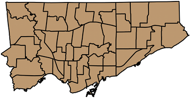
Averaging the numbers for the streets I chose gets 16.684°; just the thing for Torontohenge. For a visual axis, maybe using Steeles’s 17.194° could be better, as it’s a line above the city. You can set the map rotation angle in QGIS’s map composer, and get a better aligned city:
Categories
GIS

but where am i, really?

In my first post I asked where am i? The gps in my phone said I was standing at 43.73066°N, 79.26482°W. In real life, I was standing at the junction of Kenmark Blvd and Chevron Cres.

With the Open Toronto centreline data, I can check the location of road intersections:

select distinct (
astext (
transform (
intersection ( r1.geometry, r2.geometry ), 4326
 ) ) )
from centreline as r1, centreline as r2
where r1.lf_name = 'KENMARK BLVD' and r2.lf_name
 = 'CHEVRON CRES'

which returns:

NULL
POINT(-79.262423 43.730019)
POINT(-79.264815 43.730591)

Hmm; three answers. NULL I can’t answer; I’ll put it down as an exhortation to Be Here Now. The second is given a clue by one of the street names: Chevron Crescent – first thing I learned when I had my newspaper round is that a crescent’s going to end you up back on the same road you started from. The last one, though, agrees to 5(ish) decimal places – well within the accuracy of my simple GPS.

Update: This query gets really, really slow on long streets. Both Chevron and Kenmark only have two road segments. Kennedy and Steeles East each have over 90.

Categories
GIS

Finding the exact geographic centre of Toronto

Spacing has alluded to it. The Ontario Science Centre makes bold (and incorrect) claims about it. But here’s the real deal.

  • If you consider Toronto to be defined by its city wards, the centre of Toronto lies at 43.725518°N, 79.390531°W.
  • If you consider Toronto to be defined by its neighbourhoods, the centre of Toronto lies at 43.726495°N, 79.390641°W.

You can work this out in one line of SQL. By combining all the wards or neighbourhoods into one union shape (SpatiaLite uses the GUnion() function), and then calculating the centroid, that’s the centre of the city:

select astext(transform(centroid(gunion(geometry)),4326)) from wards

To get the results in a more human-friendly format, I transformed it to WGS84 (EPSG SRID 4326), and used astext() to get it in something other than binary.

Update, 18 March: great minds, etc … Torontoist just posted the similar In Search of Toronto’s Geographic Centre.

Categories
GIS

oooOOOooh!

Now that’s a bit better. And I did it with only mild shapefile abuse.

You can load the DBF component of a shapefile into Openoffice Calc. Columns get given headers which describe their format. By pasting in the candidates column, adding the right column definition, and then resaving, you get a shapefile with today’s candidates as a new field.

Categories
GIS

using CSV as a virtual data source

While we already know how to make trivial shapefiles with shapelib, sometimes that’s too tedious. Very frequently I get data in Comma Separated Value (CSV) format, and reliably importing/converting it can be a pain.

Here’s our sample CSV file, library_test.csv:

"Easting","Northing","Library"
625539.6,4837170.9,"Dufferin St. Clair"
625862.0,4838241.1,"Oakwood Village"
626251.0,4835287.2,"Bloor Gladstone"
626671.7,4836922.6,"Davenport"
627227.2,4840006.4,"Forest Hill"

ogr has a CSV driver. In its documentation the Virtual Format driver is touched upon. This allows you to set up a data definition file, especially useful if you read the same format frequently.

Here’s the VRT file for that CSV:

<OGRVRTDataSource>
    <!-- note that OGRVRTLayer name must be basename of source file -->
    <OGRVRTLayer name="library_test">
        <SrcDataSource>library_test.csv</SrcDataSource>
        <GeometryType>wkbPoint</GeometryType>
        <!-- your SRS goes here; I used EPSG SRID -->
        <LayerSRS>EPSG:2958</LayerSRS>
        <GeometryField encoding="PointFromColumns" x="Easting" y="Northing"/>
   </OGRVRTLayer>
</OGRVRTDataSource>

Your CSV file will now behave like a shapefile, or indeed any other geo-format that OGR understands. QGIS is a bit picky – it doesn’t seem to always work out the path of the source file.

To prove these are real coordinates, here’s what I did to make a Google Earth KML file:

ogr2ogr -f KML -t_srs EPSG:4326 library_test.kml library_test.vrt -dsco NameField=Library

Technically, you don’t need to specify the SRS for KML output as it only supports EPSG:4326, but I found you got trivially different results if it was omitted.

Try this in Google Earth: library_test.kml

Categories
GIS

ward maps: kinda working, sorta

Now I’ve sorted out formatting the labels and scraping the data, I should be almost ready to produce a pretty map.

Well, almost. The DBF component of a shapefile seems somewhat resistant to adding a column, and SQLite doesn’t seem very happy with its ALTER TABLE ADD COLUMN ... syntax.

As usual, I needed to create the database table from the shapefile. I’m not bothered about CRS, so I used -1.


.read init_spatialite-2.3.sql ASCII

.loadshp TCL3_ICITW Wards CP1252 -1

alter table wards add column candidates integer

I had mixed success getting data to load into this new column. So I improvised.

!!! WARNING: EGREGIOUS MISUSE OF DATA FOLLOWS !!!

(Sensitive readers are advised to look away)

There’s a seeming unused numeric column SHAPE_LEN in the table. As my new candidates column was coming up with occasional nulls, I cheated:


UPDATE Wards set shape_len=3 where scode_name="1"

UPDATE Wards set shape_len=1 where scode_name="2"

UPDATE Wards set shape_len=0 where scode_name="3"

...

UPDATE Wards set shape_len=3 where scode_name="44";

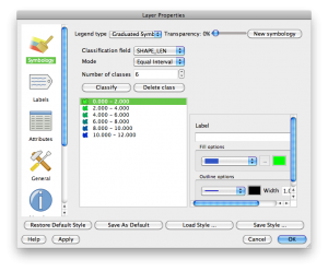
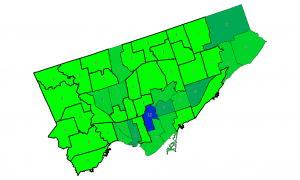
I then added SHAPE_LEN as the label, and defined a range based colour gradient for the wards in QGIS’s layer properties:

And this is how it looks:

Another partial success, as Professor Piehead would say.

Categories
GIS

closer to ward maps: scraping the data

Toronto publishes its candidates here  http://app.toronto.ca/vote2010/findByOffice.do?officeType=2&officeName=Councillor in a kind of tabular format. All I want to do is count the number of candidates per ward, remembering that some wards have no candidates yet.

Being lazy, I’d far rather have another program parse the HTML, so I work from the formatted output of W3M. It’s relatively easy to munge the output using Perl. From there, I hope to stick the additional data either into a new column in the shapefile, or use SpatiaLite. I’m undecided.

My dubious Perl script:


#!/usr/bin/perl -w
# ward_candidates - mimic mez ward map
# created by scruss on 02010/03/01
# RCS/CVS: $Id$

use strict;
my $URL =
'http://app.toronto.ca/vote2010/findByOffice.do?officeType=2&officeName=Councillor';
my $stop = 1;

my %wards;
for ( 1 .. 44 ) {
 $wards{$_} = 0;    # initialise count to zero for each ward
}

open( IN, "w3m -dump \"$URL\" |" );
while (<IN>) {
 chomp;
 s/^\s+//;
 next if (/^$/);
 $stop = 1 if (/^Withdrawn Candidate/);
 unless ( 1 == $stop ) {
 my ($ward) = /(\d+)$/;
 $wards{$ward}++;    # increment candidate for this ward
 }
 $stop = 0 if (/^City Councillor/);
}
close(IN);

foreach ( sort { $a <=> $b } ( keys(%wards) ) ) {
 printf( "%2d\t%2d\n", $_, $wards{$_} );
}

exit;

which outputs the following (header added for clarity):

Ward Candidates
==== ==========
 1     3
 2     1
 3     0
 4     0
 5     1
 6     1
 7     7
 8     3
 9     2
10     3
11     2
12     3
13     1
14     4
15     3
16     1
17     2
18     4
19     6
20     2
21     1
22     1
23     1
24     0
25     2
26     3
27    12
28     3
29     6
30     3
31     3
32     2
33     1
34     0
35     5
36     2
37     2
38     2
39     1
40     2
41     1
42     5
43     3
44     3