Categories
GIS

The highest point in Toronto

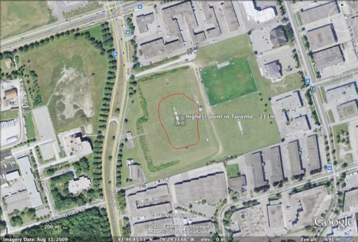
The highest point in Toronto has an elevation of 211m, and appears to be in the middle of one of York University‘s playing fields, just southwest of Keele & Steeles W:

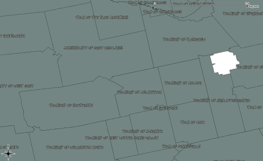
The red blob is the 211m contour, and the centre point is at 43.779325°N, 79.492655°W. The contour was derived from the MNR DEM data for the province.

The city says the highest point is 209 m (at intersection of Steeles Ave West and Keele St), which is pretty close in all three axes.

Categories
GIS

MNR DEM tiles

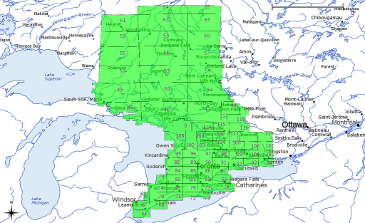
So I got the DEM tiles for my zone, couriered from Peterborough. Even zipped, they are several gigabytes. Here’s a visual guide to the tiles I got:

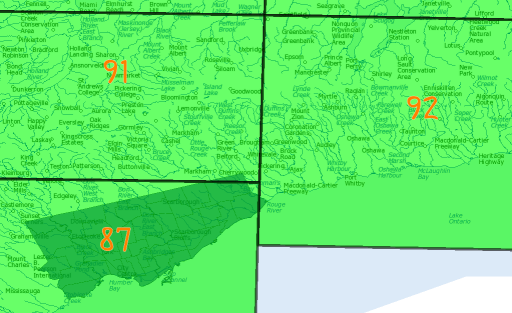
It seems that every project I work on is split across several tiles. My fair city is no exception:

Most of the city is in tile 87, but the northern and eastern corners poke into tiles 91 & 92. Merging the files and pulling out the area isn’t that hard.

First off, we need to know the extents we want. Conveniently, I’d already transformed the Open Toronto data to the same CRS, so I could just go from the extents of one of the city shape files:

$ ogrinfo -al ../open-toronto-shp/dest/2958/city-wards/TCL3_ICITW.shp | grep '^Extent'
Extent: (609538.195527, 4826360.800158) - (651613.577420, 4857439.389359)

You can then use gdal_merge.py to merge the tiles. Annoyingly, rather than using the familiar ‘lower left – upper right’ coordinate convention for bounding box, it uses ‘upper left – lower right’, so working out a buffered bounding box is a bit of a pain:

gdal_merge.py -v -of EHdr -o Toronto.flt -n -9999 -ul_lr 609000 4858000 652000 4826000 `find . -iname 'd*.flt'`

The MNR DEMs are shipped as ESRI .hdr Labelled files, 32-bit floating point. The CRS used is NAD83 Zone 17N. For all that they’re large, they’re quite quick to load and move around.

Categories
GIS

Land Information Ontario – or, how I semi-accidentally ordered 3.5GB of terrain data

The Ontario Ministry of Natural Resources has a fairly well-hidden service that provides free geodata to the general public. One has to register with a sign and e-mail form, but there’s a large number of useful data sets available. The only disadvantage is that you can’t tell if your order will be delivered by download, or physically burnt to DVD and mailed from the MNR in Peterborough. The municipalities shown above were a download; the DEMs of my entire UTM zone? They’re in the mail …

Categories
GIS

untangling CanVec

It’s almost as if NRCan doesn’t want anyone to use CanVec. I mean, it’s a free and comprehensive data set for the whole country; anyone who can type in a postal code and click a couple of times can download the CanVec map tile for where they live. But on the other hand, cracking open that download reveals an impenetrable mess of information that probably makes most users go away.

I’ve played with it before, and do occasionally drag out a layer at work, but have never got much further than that. GIS types must be very quiet, because Using CanVec – maphew and CanVec – OpenStreetMap Wiki are about the only public discussions of its content.

CanVec is delivered in two formats: Geography Markup Language (GML), and our friend, the Shapefile. While the GML version contains relatively few files, all the tools I have choke on the data. So shapefiles it is.

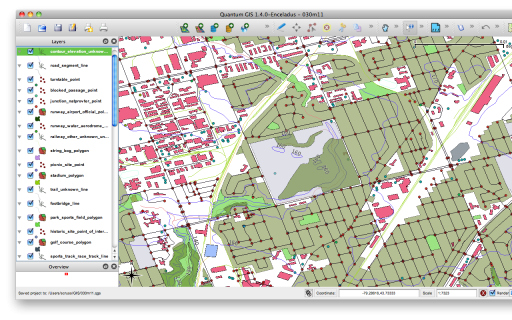
Opening up the archive for the Toronto area (it’s tile 030m11) I see 192 files. Four of those are (not very useful) metadata files. Realising that a shapefile ships as four files (the mandatory shp, dbf and shx files, plus the optional prj file) that’s 47 layers. The file names look a bit like this: 030m11_6_0_BS_1250009_0.shp, 030m11_6_0_BS_1370009_2.shp, 030m11_6_0_BS_2010009_0.shp. The names really do mean something:

030m11_6_0_BS_1370009_2.shp
|--+-| |+| |----+-----|
   |    |        \ Layer Code and Type
   |    \ Version
   \ Map tile

CanVec – Entity Names and Codes, Edition 1.1.0 (XLS) explains the layers, and how they relate to the shapefile names. Rather than relating unique layer codes to layer descriptions, the Entity Names & Codes document has it backwards. So I made the much simplified canvec_simple-20100523.csv which lists layer codes against attributes in a more sensible manner. I added a derived ‘name’ column, which I use for layer naming from these files. The layers use EPSG:4617 (NAD83 CSRS) coordinates.

Tip of the hat to maphew – Revision 123: /trunk/gis/canvec for providing a file that was the ‘Aha!’ moment.

Categories
GIS

use and abuse of elevation contours

I’d never really looked at elevation in GIS data before, mainly because the data sets are big and I didn’t understand the format. I believe that in GeoGratis, NTDB and its successor CanVec provide elevation data, but those are vector formats. Most terrain data is delivered in DEM rasters, and in Canada you can get them from GeoBase.

GeoBase DEM files come in archives containing two tiles, the east and the west. I’m not quite sure why they do this. Unless you live in an area of spectacularly interesting terrain, loading them straight into your mapping package will likely result in a large splodge of flat greyness. Because they are 2D arrays of spot heights, there’s not much variation between neighbouring points, unless you’re at a cliff.

Another issue you need to address in reading DEM files is the handling of unknown values. gdalinfo will show you the value in a line like

NoData Value=-32767

Unless you filter that value out, your DEM file will appear to have holes approximately 4x the height of Everest. This causes problems if you try to make a colour map.

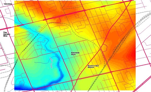
Here’s the DEM for my neighbourhood, translated and cropped using gdalwarp, and false-coloured in QGIS:

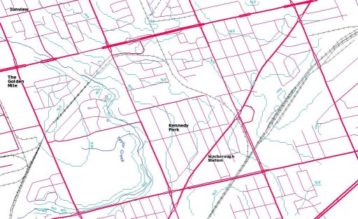
Not surprisingly, Taylor Creek runs through the lowest ground (funny how water does that …). I could have picked off spot heights with QGIS’s ‘Identify Features’ tool, but contours are neater:

I made the 5m contours with gdal_contour, using the following command (on the terrain data which I’d converted to GeoTIFF):

gdal_contour -a elev -3d kennedy_park.tif kennedy_park-contours.shp -i 5.0 -snodata -32767

Looking at that map, and despite the somewhat wibbly nature of raster-vector converted contours, the elevation of my house is about 167m. My GPS – a Garmin GPSMAP 60CSx – contains a barometric pressure sensor, and on a day I’d remembered to calibrate it by the lake, it said I was at 166.9m above sea level. Neato!

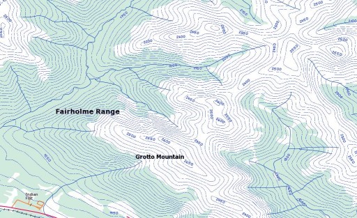
Update: just to show that Canada has some wiggly bits, here are some contours for Grotto Mountain, not far from Canmore, AB:

These are 50m contours, though – 5m would just be a blur.

Categories
Uncategorized

Taking geotagged pictures with your Blackberry

Note: I’ve had reports that some carriers seem to disable GPS service within their service area. I’ve certainly seen slight differences as to how this works on different carriers.

Most recent camera-equipped Blackberrys have a GPS built in. One of the most handy things I’ve found for fieldwork is the ability to take pictures tagged with your location and be able to send them to contacts.

Setting this up is a little involved. First, go into the camera, and selection ‘Camera Options’. You want to enable Geotagging:

(oh, and I took the screen capture with CaptureIt). Save options, then exit back to the home screen.

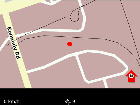
I find the most reliable way of starting the GPS is to go into Blackberry Maps, and ‘Start GPS Navigation’ from the menu. Once you’ve got a reliable satellite fix (which on my old Curve, used to work fine indoors; on my Tour, not so well) you should be able see the map update with your current location, and a satellite count (9 here) on the bottom of the screen:
Exit maps, and start your camera. You’ll know if you have a location for tagging if there’s an icon that looks a bit like  in the bottom right corner of the screen. With no fix, it’s a red crossed-through icon. Now take your picture!
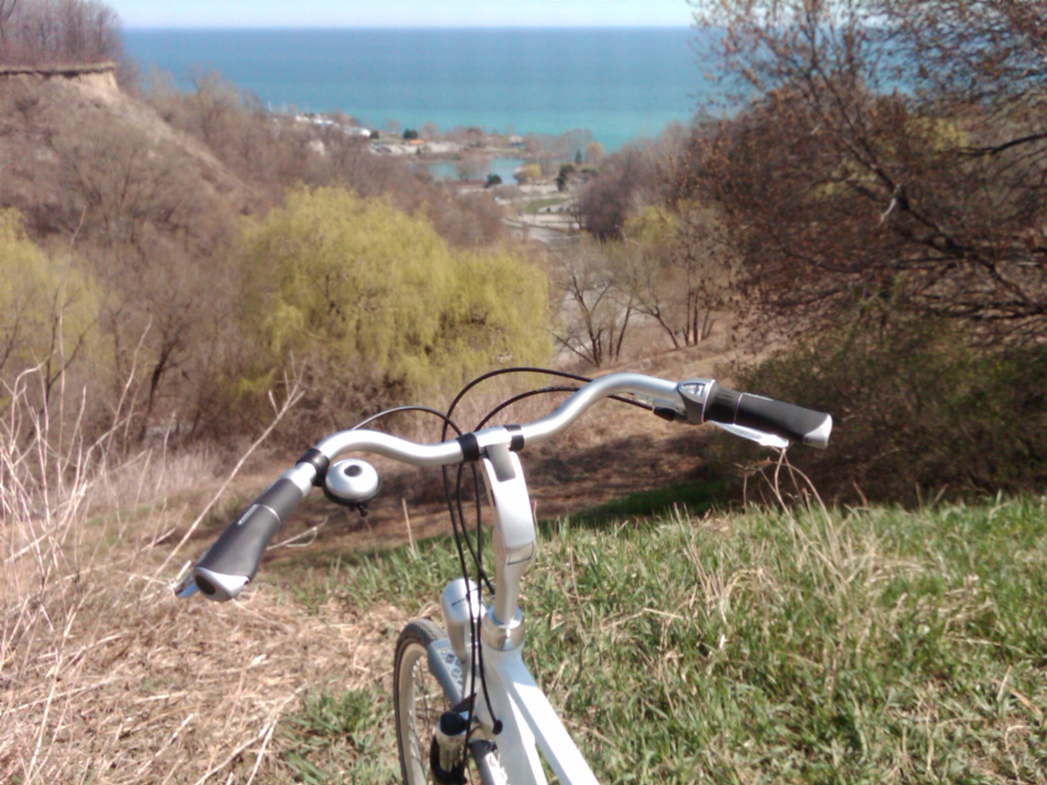
(yeah, my Blackberry takes slightly fuzzy pictures. Dunno why.)

Metadata’s only useful if you can read it, and on anything with a command line, ExifTool works really well:

$ exiftool IMG00144-20100411-1516.jpg
 ...
GPS Position                    : 43.709983 N, 79.239817 W

(one should note that without a barometric pressure sensor, GPS altitude readings are not to be trusted. This picture claimed to be taken at 120 m Below Sea Level …)

Curiously, OS X’s Preview gets GPS position completely wrong:
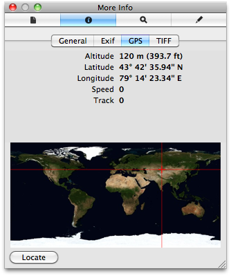
According to Preview, I and my bike (and my Blackberry) were close to Charyn in Kazakhstan. I’m quick on my pedals, but not good enough to get far east in an afternoon.

iPhoto gets it right, though:
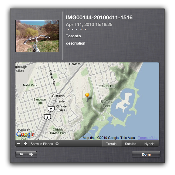
Curiously, I couldn’t find anything built into Windows (okay, XP) that would read the tag location. I guess Microsoft just don’t want you to know where you are now, merely where do you want to go today.
Categories
GIS

three norths to choose from

North is a slippery thing, a trickster. There are at least three norths to choose from:

  • Magnetic north – where the compass needle points. Currently way in the northwest of Canada, it’s scooting rapidly towards Siberia. Come baaack, magnetic north! Was it something we said?
  • True north – straight up and down on the axis of this planet.
  • Grid north – the vertical lines on your map. Due to the earth’s curvature, there’s only one line on a grid that exactly coincides with true north. Away from that line, there’s a correction that you need to apply.

That grid to true correction is what I’m looking at today. In my work, I need to work out where shadows of wind turbines fall. I work in grid coordinates, so I need to correct for true north sun angles. Here’s a shell script that uses familiar programs invproj and geod to work out the local true north correction:

#!/bin/sh
# gridnorth.sh - show the grid shift angle at a certain point
# created by scruss on Sun 4 Apr 2010 18:19:29 EDT
# $Id: gridnorth.sh,v 1.2 2010/04/05 12:23:57 scruss Exp $

# you might want to change this
srid=2958

# two arguments mandatory, third optional
if
 [ $# -lt 2 ]
then
 echo Usage: $0 x y [srid]
fi

# truncate arguments to integers so the shell maths will work
x=`echo $1 | sed 's/\.[0-9]*//;'`
y=`echo $2 | sed 's/\.[0-9]*//;'`
# calculate points 1000 units (grid) south and north of the chosen point
lowy=$((y-1000))
highy=$((y+1000))

if
 [ $# -eq 3 ]
then
 srid=$3
fi

min=`echo $lowy  $x foo | invproj -r -f "%.6f" +init=EPSG:$srid`
max=`echo $highy $x foo | invproj -r -f "%.6f" +init=EPSG:$srid`
minlon=`echo $min | awk '{print $1;}'`
minlat=`echo $min | awk '{print $2;}'`
maxlon=`echo $max | awk '{print $1;}'`
maxlat=`echo $max | awk '{print $2;}'`
echo $minlat $minlon $maxlat $maxlon |\
 geod +ellps=WGS84 -f "%.3f" -p -I +units=m |\
 awk '{print $1;}'

The script is called with two arguments (the easting and the northing) and an optional third argument, the SRID for the current projection:

$ ./gridnorth.sh 639491 4843599 26717
1.198

The value returned is the angle (clockwise) that grid north differs from true north. Unless you’re using the same SRID that I’ve put in the script as default, you probably want to specify (or change) it.

So how do I know if this is even remotely correct? If you look at any CanMatrix scanned topographic map (either Print Ready or Georeferenced). there’s a declination indicator shown:

That’s the map eastern Toronto is in; its sheet reference is 030M11. We’ll ignore the magnetic declination for now, as 1984 is way out of date, and there is much to be said on geomagnetism that I don’t understand.  The map says its centre is 1° 12′ clockwise of true north. The centre of the map is approximately 641500E, 4831000N (UTM Zone 17N NAD27; EPSG 26717; or in real terms, in the lake, a few klicks SE of Ashbridges Bay) so:

$ ./gridnorth.sh 641500 4831000 26717
1.209

1° 12′ is 1.2, so I think I’m officially pretty durn close.

To show that grid skew changes across the map, the upper right hand corner of the map is 660000E, 4845000N, which is off by 1.375°.

Categories
Uncategorized

current tools of my trade

Mark asked: What kind of GIS software are you using?
Well, since you asked:-

  • SpatiaLite: spatial awesome built on SQLite. I love it because I don’t need to play DBA.
  • QGIS: for maps
  • ogr: for file format futzing
  • proj: for scrupulously correct (well, if I knew what I was doing …) conversion between projected and otherwise.
  • OpenOffice: for those tedious calculations
  • … and about 20 years of unix experience to mash all the results together.

All of the above are free. I’m doing this because I want to learn. Asking elsewhere hasn’t turned up anything useful.

Categories
GIS

Toronto’s Human Centre, part 2: by neighbourhood

Beware throwaway comments; that way overanalysis lies. This was a challenge.

Taking the 2006 neighbourhoods population into account, the human centre of Toronto is at 43.717955°N, 79.389828°W …

… pretty close to the one I’ve already worked out by ward.

Scraping the neighbourhood populations was hard. For the 140 neighbourhoods, the data is stored in a pdf with the URL like http://www.toronto.ca/demographics/cns_profiles/2006/pdf1/cpa124.pdf (in this case, 124; Kennedy Park, represent!). The population number is stored in a table on page 2 of each pdf. I used pdf2xml to convert the files into something parseable.

Of course, the tables weren’t exactly in the same place in every file, so I took a sample of 10% of the files, and worked out the X & Y coordinates of the population box. pdf2xml spits out elements like

<TOKEN sid="p2_s427" id="p2_w417" font-name="arialmt" serif="yes" fixed-width="yes" bold="no" italic="no" font-size="7.47183" font-color="#000000" rotation="0" angle="0" x="299.739" y="122.117" base="129.634" width="22.7692" height="9.94501">17,050</TOKEN>

Yes, I should have used an XML parser, but a Small Matter of Perl got me 126 out of the 140 matching. The rest I keyed in by hand …

Table after the jump.

Categories
GIS

finding the nearest thing to another thing

Something I used to have to do a lot was to maintain a table of the nearest houses to prospective wind farm layouts. While the list of houses didn’t change very much, the layouts did. I came up with an only semi-unwieldy spreadsheet to do the calculations. The table was ultimately used in submissions to the Ontario Ministry of the Environment.

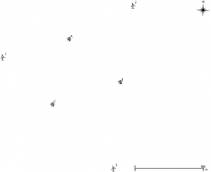
I’ve mapped out a trivially small example below; three houses, three wind turbines. In real life, there would be hundreds of each.

Sorry to include it as an image, but WordPress really doesn’t like pasted tables. If you really must, the text content is below the fold.

Though it’s small, it’s a bit of a horror, so you might want to download near.ods (opendocument spreadsheet). The mauve section contains the house coordinates, the blue the turbines. The green section is a simple Cartesian distance calculator (√(Δx2+Δy2)) for those coordinates. The beige (or orange; or is it salmon?) bit is where things get difficult. Finding the closest distance is easy with the MIN function. Finding the column heading in which that minimum distance occurs is a bit more tricky, using INDIRECT, ADDRESS, COLUMN and MATCH to pull out the contents of the cell. This is one of the few spreadsheets I’ve written that will break if you rearrange it; hardcoded cell address mathematics will do that.

Getting the same result in SQL is little more difficult. I mean, I can make the table of distances easily enough:


select houses.ref as House,
 turbines.id as Turbine,
 distance(houses.geom, turbines.geom) as Distance
from houses, turbines
order by House, Turbine

but producing a nice compact table of houses, the nearest turbine, and the distance will need more pondering.