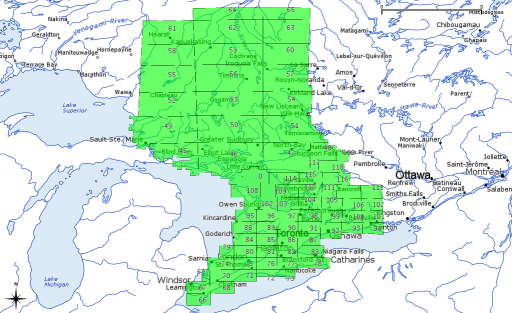
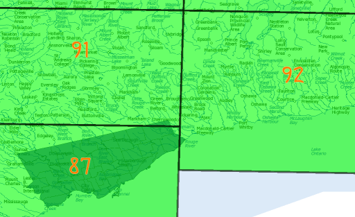
I’d never really looked at elevation in GIS data before, mainly because the data sets are big and I didn’t understand the format. I believe that in GeoGratis, NTDB and its successor CanVec provide elevation data, but those are vector formats. Most terrain data is delivered in DEM rasters, and in Canada you can get them from GeoBase.
GeoBase DEM files come in archives containing two tiles, the east and the west. I’m not quite sure why they do this. Unless you live in an area of spectacularly interesting terrain, loading them straight into your mapping package will likely result in a large splodge of flat greyness. Because they are 2D arrays of spot heights, there’s not much variation between neighbouring points, unless you’re at a cliff.
Another issue you need to address in reading DEM files is the handling of unknown values. gdalinfo will show you the value in a line like
NoData Value=-32767
Unless you filter that value out, your DEM file will appear to have holes approximately 4x the height of Everest. This causes problems if you try to make a colour map.
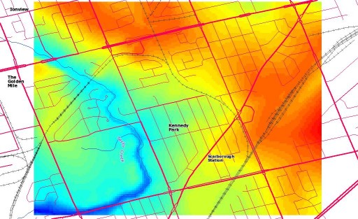
Here’s the DEM for my neighbourhood, translated and cropped using gdalwarp, and false-coloured in QGIS:

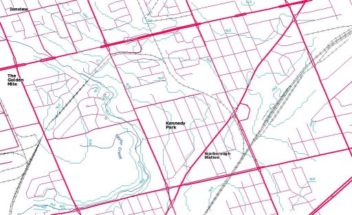
Not surprisingly, Taylor Creek runs through the lowest ground (funny how water does that …). I could have picked off spot heights with QGIS’s ‘Identify Features’ tool, but contours are neater:

I made the 5m contours with gdal_contour, using the following command (on the terrain data which I’d converted to GeoTIFF):
gdal_contour -a elev -3d kennedy_park.tif kennedy_park-contours.shp -i 5.0 -snodata -32767
Looking at that map, and despite the somewhat wibbly nature of raster-vector converted contours, the elevation of my house is about 167m. My GPS – a Garmin GPSMAP 60CSx – contains a barometric pressure sensor, and on a day I’d remembered to calibrate it by the lake, it said I was at 166.9m above sea level. Neato!
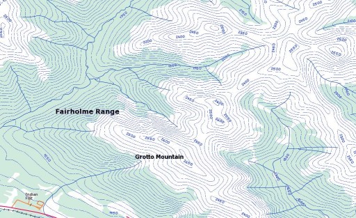
Update: just to show that Canada has some wiggly bits, here are some contours for Grotto Mountain, not far from Canmore, AB:
 These are 50m contours, though – 5m would just be a blur.
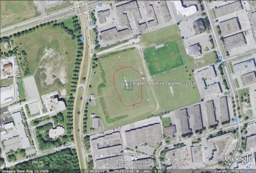 The red blob is the 211m contour, and the centre point is at 43.779325°N, 79.492655°W. The contour was derived from the MNR DEM data for the province.