Categories
GIS

untangling CanVec

It’s almost as if NRCan doesn’t want anyone to use CanVec. I mean, it’s a free and comprehensive data set for the whole country; anyone who can type in a postal code and click a couple of times can download the CanVec map tile for where they live. But on the other hand, cracking open that download reveals an impenetrable mess of information that probably makes most users go away.

I’ve played with it before, and do occasionally drag out a layer at work, but have never got much further than that. GIS types must be very quiet, because Using CanVec – maphew and CanVec – OpenStreetMap Wiki are about the only public discussions of its content.

CanVec is delivered in two formats: Geography Markup Language (GML), and our friend, the Shapefile. While the GML version contains relatively few files, all the tools I have choke on the data. So shapefiles it is.

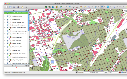
Opening up the archive for the Toronto area (it’s tile 030m11) I see 192 files. Four of those are (not very useful) metadata files. Realising that a shapefile ships as four files (the mandatory shp, dbf and shx files, plus the optional prj file) that’s 47 layers. The file names look a bit like this: 030m11_6_0_BS_1250009_0.shp, 030m11_6_0_BS_1370009_2.shp, 030m11_6_0_BS_2010009_0.shp. The names really do mean something:

030m11_6_0_BS_1370009_2.shp
|--+-| |+| |----+-----|
   |    |        \ Layer Code and Type
   |    \ Version
   \ Map tile

CanVec – Entity Names and Codes, Edition 1.1.0 (XLS) explains the layers, and how they relate to the shapefile names. Rather than relating unique layer codes to layer descriptions, the Entity Names & Codes document has it backwards. So I made the much simplified canvec_simple-20100523.csv which lists layer codes against attributes in a more sensible manner. I added a derived ‘name’ column, which I use for layer naming from these files. The layers use EPSG:4617 (NAD83 CSRS) coordinates.

Tip of the hat to maphew – Revision 123: /trunk/gis/canvec for providing a file that was the ‘Aha!’ moment.
Categories
GIS

use and abuse of elevation contours

I’d never really looked at elevation in GIS data before, mainly because the data sets are big and I didn’t understand the format. I believe that in GeoGratis, NTDB and its successor CanVec provide elevation data, but those are vector formats. Most terrain data is delivered in DEM rasters, and in Canada you can get them from GeoBase.

GeoBase DEM files come in archives containing two tiles, the east and the west. I’m not quite sure why they do this. Unless you live in an area of spectacularly interesting terrain, loading them straight into your mapping package will likely result in a large splodge of flat greyness. Because they are 2D arrays of spot heights, there’s not much variation between neighbouring points, unless you’re at a cliff.

Another issue you need to address in reading DEM files is the handling of unknown values. gdalinfo will show you the value in a line like

NoData Value=-32767

Unless you filter that value out, your DEM file will appear to have holes approximately 4x the height of Everest. This causes problems if you try to make a colour map.

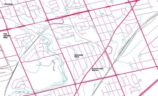
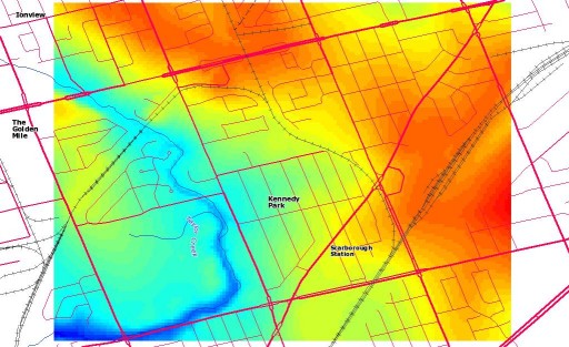
Here’s the DEM for my neighbourhood, translated and cropped using gdalwarp, and false-coloured in QGIS:

Not surprisingly, Taylor Creek runs through the lowest ground (funny how water does that …). I could have picked off spot heights with QGIS’s ‘Identify Features’ tool, but contours are neater:

I made the 5m contours with gdal_contour, using the following command (on the terrain data which I’d converted to GeoTIFF):

gdal_contour -a elev -3d kennedy_park.tif kennedy_park-contours.shp -i 5.0 -snodata -32767

Looking at that map, and despite the somewhat wibbly nature of raster-vector converted contours, the elevation of my house is about 167m. My GPS – a Garmin GPSMAP 60CSx – contains a barometric pressure sensor, and on a day I’d remembered to calibrate it by the lake, it said I was at 166.9m above sea level. Neato!

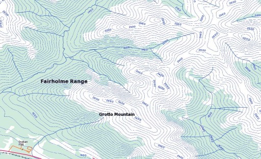
Update: just to show that Canada has some wiggly bits, here are some contours for Grotto Mountain, not far from Canmore, AB:

These are 50m contours, though – 5m would just be a blur.

Categories
GIS

three norths to choose from

North is a slippery thing, a trickster. There are at least three norths to choose from:

  • Magnetic north – where the compass needle points. Currently way in the northwest of Canada, it’s scooting rapidly towards Siberia. Come baaack, magnetic north! Was it something we said?
  • True north – straight up and down on the axis of this planet.
  • Grid north – the vertical lines on your map. Due to the earth’s curvature, there’s only one line on a grid that exactly coincides with true north. Away from that line, there’s a correction that you need to apply.

That grid to true correction is what I’m looking at today. In my work, I need to work out where shadows of wind turbines fall. I work in grid coordinates, so I need to correct for true north sun angles. Here’s a shell script that uses familiar programs invproj and geod to work out the local true north correction:

#!/bin/sh
# gridnorth.sh - show the grid shift angle at a certain point
# created by scruss on Sun 4 Apr 2010 18:19:29 EDT
# $Id: gridnorth.sh,v 1.2 2010/04/05 12:23:57 scruss Exp $

# you might want to change this
srid=2958

# two arguments mandatory, third optional
if
 [ $# -lt 2 ]
then
 echo Usage: $0 x y [srid]
fi

# truncate arguments to integers so the shell maths will work
x=`echo $1 | sed 's/\.[0-9]*//;'`
y=`echo $2 | sed 's/\.[0-9]*//;'`
# calculate points 1000 units (grid) south and north of the chosen point
lowy=$((y-1000))
highy=$((y+1000))

if
 [ $# -eq 3 ]
then
 srid=$3
fi

min=`echo $lowy  $x foo | invproj -r -f "%.6f" +init=EPSG:$srid`
max=`echo $highy $x foo | invproj -r -f "%.6f" +init=EPSG:$srid`
minlon=`echo $min | awk '{print $1;}'`
minlat=`echo $min | awk '{print $2;}'`
maxlon=`echo $max | awk '{print $1;}'`
maxlat=`echo $max | awk '{print $2;}'`
echo $minlat $minlon $maxlat $maxlon |\
 geod +ellps=WGS84 -f "%.3f" -p -I +units=m |\
 awk '{print $1;}'

The script is called with two arguments (the easting and the northing) and an optional third argument, the SRID for the current projection:

$ ./gridnorth.sh 639491 4843599 26717
1.198

The value returned is the angle (clockwise) that grid north differs from true north. Unless you’re using the same SRID that I’ve put in the script as default, you probably want to specify (or change) it.

So how do I know if this is even remotely correct? If you look at any CanMatrix scanned topographic map (either Print Ready or Georeferenced). there’s a declination indicator shown:

That’s the map eastern Toronto is in; its sheet reference is 030M11. We’ll ignore the magnetic declination for now, as 1984 is way out of date, and there is much to be said on geomagnetism that I don’t understand.  The map says its centre is 1° 12′ clockwise of true north. The centre of the map is approximately 641500E, 4831000N (UTM Zone 17N NAD27; EPSG 26717; or in real terms, in the lake, a few klicks SE of Ashbridges Bay) so:

$ ./gridnorth.sh 641500 4831000 26717
1.209

1° 12′ is 1.2, so I think I’m officially pretty durn close.

To show that grid skew changes across the map, the upper right hand corner of the map is 660000E, 4845000N, which is off by 1.375°.

Categories
GIS

Toronto’s Human Centre, part 2: by neighbourhood

Beware throwaway comments; that way overanalysis lies. This was a challenge.

Taking the 2006 neighbourhoods population into account, the human centre of Toronto is at 43.717955°N, 79.389828°W …

… pretty close to the one I’ve already worked out by ward.

Scraping the neighbourhood populations was hard. For the 140 neighbourhoods, the data is stored in a pdf with the URL like http://www.toronto.ca/demographics/cns_profiles/2006/pdf1/cpa124.pdf (in this case, 124; Kennedy Park, represent!). The population number is stored in a table on page 2 of each pdf. I used pdf2xml to convert the files into something parseable.

Of course, the tables weren’t exactly in the same place in every file, so I took a sample of 10% of the files, and worked out the X & Y coordinates of the population box. pdf2xml spits out elements like

<TOKEN sid="p2_s427" id="p2_w417" font-name="arialmt" serif="yes" fixed-width="yes" bold="no" italic="no" font-size="7.47183" font-color="#000000" rotation="0" angle="0" x="299.739" y="122.117" base="129.634" width="22.7692" height="9.94501">17,050</TOKEN>

Yes, I should have used an XML parser, but a Small Matter of Perl got me 126 out of the 140 matching. The rest I keyed in by hand …

Table after the jump.

Categories
GIS

finding the nearest thing to another thing

Something I used to have to do a lot was to maintain a table of the nearest houses to prospective wind farm layouts. While the list of houses didn’t change very much, the layouts did. I came up with an only semi-unwieldy spreadsheet to do the calculations. The table was ultimately used in submissions to the Ontario Ministry of the Environment.

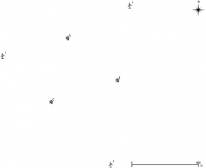
I’ve mapped out a trivially small example below; three houses, three wind turbines. In real life, there would be hundreds of each.

Sorry to include it as an image, but WordPress really doesn’t like pasted tables. If you really must, the text content is below the fold.

Though it’s small, it’s a bit of a horror, so you might want to download near.ods (opendocument spreadsheet). The mauve section contains the house coordinates, the blue the turbines. The green section is a simple Cartesian distance calculator (√(Δx2+Δy2)) for those coordinates. The beige (or orange; or is it salmon?) bit is where things get difficult. Finding the closest distance is easy with the MIN function. Finding the column heading in which that minimum distance occurs is a bit more tricky, using INDIRECT, ADDRESS, COLUMN and MATCH to pull out the contents of the cell. This is one of the few spreadsheets I’ve written that will break if you rearrange it; hardcoded cell address mathematics will do that.

Getting the same result in SQL is little more difficult. I mean, I can make the table of distances easily enough:


select houses.ref as House,
 turbines.id as Turbine,
 distance(houses.geom, turbines.geom) as Distance
from houses, turbines
order by House, Turbine

but producing a nice compact table of houses, the nearest turbine, and the distance will need more pondering.

Categories
GIS

toronto’s human centre

Since it was trivial to calculate the centre of the city, I thought I’d do something a little more complex: calculate the centre of the city, weighted for population. I scraped the 2006 population data by ward from the City of Toronto: Ward Profiles pages; hooray for curl and regexes. Realising that I had no information on population distribution within wards, I made a good old engineering assumption: we could idealize the population as a point mass at the centroid of each ward, and then calculate the centre of mass by balancing moments around the X and Y axis. (I mean, c’mon – it’s the sort of thing we all think about daily … isn’t it? Guys … hello … anyone there?)

I’ll spare you the details until after the jump, but I calculate the human centre of Toronto to be at 43.717794°N, 79.390299°W – that’s in Blythwood Ravine, just south of Blythwood Road. We should have a picnic there …

Categories
GIS

a minor revelation about road segments

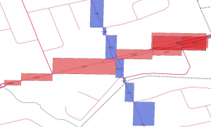
I’m still learning how Toronto encodes its roads – and whether this is a common practice. Between intersections, roads are stored as polyline segments. Kennedy Road (blue) and Eglinton Ave E (red) are shown below as a series of road segment minimum bounding rectangles (MBR):


I was hoping it would be quick and easy to find the MBR of the whole street, then search for intersections only in the intersections of the MBRs. On an orthogonal grid (even a squinty one) this would save a bunch of searching.

I don’t know if I can use the fact that the end points of road sections are common at intersections. I really am a geonumpty.

All this may soon be moot, as I hear that the next release of the toronto.ca | Open data – expected early April – will have explicit intersection data. Yay!

Categories
GIS

Toronto’s Angles

As many Canadians will tell you, most Torontonians are a bit skewed. While others might have different explanations, I put it down to our road grid. What we call north in the city is actually some 16.7° west of north.

While we do have a perpendicular grid, it’s twisted to the left (steady, Edmontonians). I attempted to work out what the average angle is.

I eyeballed several long straight streets, and picked out representative intersections. Finidng the coordinates of these intersections took a surprisingly long time, as each street has several road sections. To find an intersection, each section on one road has to be queried against each section of the other. It gets there, eventually.

To save the tedium of showing the queries, here are the results. The angles are anticlockwise from the X-axis.

N-S	 Intersection1 Intersection2 Angle
======== ============= ============= ======
Bathurst King	       Dupont	     16.184
Yonge	 King	       Rosehill	     16.783
Woodbine Queen	       Plains	     17.049

E-W	 Intersection1 Intersection2 Angle
======== ============= ============= ======
Danforth Greenwood     Main	     16.736
Eglinton Dufferin      Bayview	     16.159
Steeles	 Dufferin      Kennedy	     17.194

I was surprised that SpatiaLite didn’t have any angle measurement functions built in, so I had to feed the output through geod. So for instance, for Steeles Avenue, the intersection of Steeles West and Dufferin is at 43.787229°N, 79.470285°W, and the intersection of Steeles East and Kennedy is 43.823636°N, 79.307265°W. Feeding these numbers to geod:

echo '43.787229 -79.470285 43.823636 -79.307265'| geod +ellps=WGS84 -f &quot;%.3f&quot; -p -I +units=m

This spits out three numbers: 72.806    252.918    13727.395. The first is the bearing from the first point to the second; this is the number we’re interested in, and it’s (90-82.806) = 17.194° clockwise from E. The second is the bearing from the second point back to the first. The last is the distance in metres; Steeles is a long, straight street.

Averaging the numbers for the streets I chose gets 16.684°; just the thing for Torontohenge. For a visual axis, maybe using Steeles’s 17.194° could be better, as it’s a line above the city. You can set the map rotation angle in QGIS’s map composer, and get a better aligned city:

Categories
GIS

but where am i, really?

In my first post I asked where am i? The gps in my phone said I was standing at 43.73066°N, 79.26482°W. In real life, I was standing at the junction of Kenmark Blvd and Chevron Cres.

With the Open Toronto centreline data, I can check the location of road intersections:

select distinct (
astext (
transform (
intersection ( r1.geometry, r2.geometry ), 4326
 ) ) )
from centreline as r1, centreline as r2
where r1.lf_name = 'KENMARK BLVD' and r2.lf_name
 = 'CHEVRON CRES'

which returns:

NULL
POINT(-79.262423 43.730019)
POINT(-79.264815 43.730591)

Hmm; three answers. NULL I can’t answer; I’ll put it down as an exhortation to Be Here Now. The second is given a clue by one of the street names: Chevron Crescent – first thing I learned when I had my newspaper round is that a crescent’s going to end you up back on the same road you started from. The last one, though, agrees to 5(ish) decimal places – well within the accuracy of my simple GPS.

Update: This query gets really, really slow on long streets. Both Chevron and Kenmark only have two road segments. Kennedy and Steeles East each have over 90.

Categories
GIS

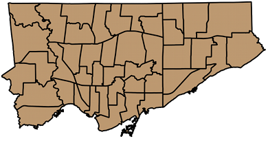
Finding the exact geographic centre of Toronto

Spacing has alluded to it. The Ontario Science Centre makes bold (and incorrect) claims about it. But here’s the real deal.

  • If you consider Toronto to be defined by its city wards, the centre of Toronto lies at 43.725518°N, 79.390531°W.
  • If you consider Toronto to be defined by its neighbourhoods, the centre of Toronto lies at 43.726495°N, 79.390641°W.

You can work this out in one line of SQL. By combining all the wards or neighbourhoods into one union shape (SpatiaLite uses the GUnion() function), and then calculating the centroid, that’s the centre of the city:

select astext(transform(centroid(gunion(geometry)),4326)) from wards

To get the results in a more human-friendly format, I transformed it to WGS84 (EPSG SRID 4326), and used astext() to get it in something other than binary.

Update, 18 March: great minds, etc … Torontoist just posted the similar In Search of Toronto’s Geographic Centre.